Graphical Method of Solving LPP

The Feasible Region and Convexity

The graphical method is used to solve a Linear Programming Problem involving two decision variables. Since only two variables are involved, the constraints can be represented on a Cartesian plane.

• Feasible Region: The common region that satisfies all the given constraints, including the non-negativity constraints $x \ge 0$ and $y \ge 0$, is called the feasible region or solution region. Every point in this region represents a feasible solution.
• Infeasible Region: Any point lying outside the feasible region violates at least one constraint and is therefore called an infeasible solution.
• Feasible Solution: Any point that satisfies all constraints.
• Optimal Feasible Solution: A feasible solution for which the objective function attains its maximum or minimum value.
• Convexity: The feasible region formed by linear constraints is always a convex region. A region is convex if, for any two points inside it, the line segment joining them lies entirely inside the region.

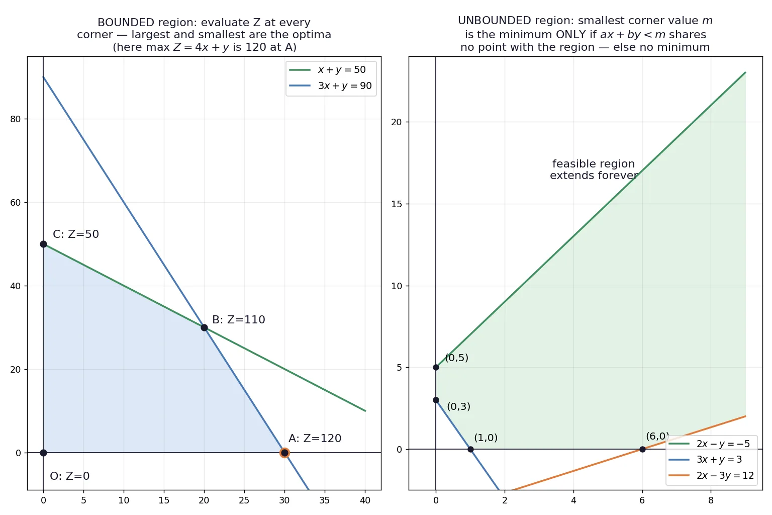
When the feasible region is enclosed by line segments, it forms a convex polygon. In some cases, the feasible region may also be unbounded, but it is still convex.

2. Fundamental Theorems of Linear Programming

The graphical method is based on two important results:

Theorem 1 (Corner Point Principle)

If a Linear Programming Problem has an optimal solution, then at least one such optimal solution occurs at a corner point (vertex) of the feasible region.

This means that instead of testing infinitely many feasible points, we only need to check the corner points of the feasible region.

Theorem 2 (Bounded Feasible Region)

If the feasible region is bounded, then the objective function definitely attains both a maximum value and a minimum value, and these occur at corner points of the feasible region.

Important Note:

If the feasible region is unbounded, an optimal solution may or may not exist. In such cases, the values at corner points alone are not always enough, especially for maximization or minimization in the direction of the unbounded part.

The Corner Point Method

To solve a two-variable LPP graphically, we use the Corner Point Method.

Step 1: Draw the boundary lines

Replace each inequality by an equality and draw the corresponding straight line.

Step 2: Identify the correct half-planes

For each inequality, determine which side of the line satisfies the condition. This is usually done by testing a convenient point such as $(0,0)$, provided the line does not pass through the origin.

Step 3: Obtain the feasible region

The common part of all valid half-planes, along with the non-negativity restrictions, gives the feasible region.

Step 4: Find all corner points

Locate all the vertices of the feasible region. If necessary, solve pairs of equations algebraically to find exact coordinates.

Step 5: Evaluate the objective function

Substitute each corner point into the objective function $Z = ax + by$.

Step 6: Identify the optimum value

• The largest value gives the maximum.
• The smallest value gives the minimum.

This method works because of the fundamental theorem that the optimum occurs at a corner point whenever it exists.

Handling Unbounded Regions

When the feasible region is unbounded, the objective function may still have an optimum, or it may fail to have one.

Suppose the corner-point evaluation gives:

• largest value $M$ for a maximization problem,
• smallest value $m$ for a minimization problem.

Then we proceed as follows:

For Maximization:

Consider the open half-plane $$ax + by > M.$$

• If this region has no common point with the feasible region, then $M$ is the maximum value.
• If it has even one common point, then the objective function can become larger than $M$, so no maximum value exists.

For Minimization:

Consider the open half-plane $$ax + by < m.$$

• If this region has no common point with the feasible region, then $m$ is the minimum value.
• If it has a common point with the feasible region, then the objective function can become smaller than $m$, so no minimum value exists.

Thus, for unbounded regions, corner points give a candidate answer, but a further check is necessary.

Special Cases in Graphical Solutions

There are some important special cases in graphical LPP:

• Multiple Optimal Solutions: If the objective function has the same optimal value at two adjacent corner points, then every point on the line segment joining those points also gives the same optimal value.
• Infeasible Problem: If there is no common region satisfying all constraints, then the feasible region is empty and the problem has no feasible solution.
• Redundant Constraint: A constraint is called redundant if removing it does not change the feasible region. It does not affect the final solution.
• Unique Optimal Solution: If the objective function has a distinct best value at only one corner point, then the solution is unique.

These cases are frequently asked in theory as well as problem-solving questions.

Example 1: Bounded Maximization

Maximize $Z = 3x + 4y$ subject to the constraints: $x + y \le 4$, $x \ge 0$, $y \ge 0$.

Solution: Step 1: Draw the line $x + y = 4$. It passes through $(4,0)$ and $(0,4)$.

Step 2: Since $x+y\le4$, the required half-plane is the one containing the origin because $(0,0)$ satisfies the inequality.

Step 3: Along with $x\ge0$ and $y\ge0$, the feasible region lies in the first quadrant under the line $x+y=4$.

Step 4: The corner points of the feasible region are:

• $O(0,0)$
• $A(4,0)$
• $B(0,4)$

Step 5: Evaluate the objective function at each corner point:

• At $O(0,0)$: $$Z = 3(0)+4(0)=0$$
• At $A(4,0)$: $$Z = 3(4)+4(0)=12$$
• At $B(0,4)$: $$Z = 3(0)+4(4)=16$$

Step 6: The largest value is $16$.

Answer: Maximum value of $Z$ is $$16$$ at the point $$(0,4).$$

Example 2: Bounded Minimization

Minimize $Z = -3x + 4y$ subject to $x + 2y \le 8$, $3x + 2y \le 12$, $x \ge 0$, $y \ge 0$.

Solution: Step 1: Draw the lines:

• $x+2y=8$, passing through $(8,0)$ and $(0,4)$
• $3x+2y=12$, passing through $(4,0)$ and $(0,6)$

Step 2: Since both inequalities are of type $\le$, the feasible region lies below both lines in the first quadrant.

Step 3: Find the corner points.

• $O(0,0)$
• $A(4,0)$ from the line $3x+2y=12$ on the x-axis
• $C(0,4)$ from the line $x+2y=8$ on the y-axis
• Intersection point of the two lines: $$x+2y=8$$ $$3x+2y=12$$ Subtracting, we get $$2x=4 \Rightarrow x=2.$$ Substituting into $x+2y=8$: $$2+2y=8 \Rightarrow 2y=6 \Rightarrow y=3.$$ So the intersection point is $$B(2,3).$$

Step 4: Evaluate $Z$ at all corner points:

• At $O(0,0)$: $$Z=0$$
• At $A(4,0)$: $$Z=-3(4)+4(0)=-12$$
• At $B(2,3)$: $$Z=-3(2)+4(3)=-6+12=6$$
• At $C(0,4)$: $$Z=-3(0)+4(4)=16$$

Step 5: The minimum among these is $-12$.

Answer: Minimum value of $Z$ is $$-12$$ at the point $$(4,0).$$

Example 3: Unbounded Minimization

Minimize $Z = 3x + 5y$ subject to $x + 3y \ge 3$, $x + y \ge 2$, $x \ge 0$, $y \ge 0$.

Solution: Step 1: Draw the boundary lines:

• $x+3y=3$, passing through $(3,0)$ and $(0,1)$
• $x+y=2$, passing through $(2,0)$ and $(0,2)$

Step 2: Since the inequalities are of type $\ge$, the feasible region lies above both lines in the first quadrant.

Step 3: The feasible region is unbounded.

Step 4: Determine the corner points of the feasible region boundary.

• Point $A(3,0)$
• Point $C(0,2)$
• Intersection of the two lines: $$x+3y=3$$ $$x+y=2$$ Subtracting gives $$2y=1 \Rightarrow y=\frac{1}{2}.$$ Then $$x=2-\frac{1}{2}=\frac{3}{2}.$$ So, $$B\left(\frac{3}{2},\frac{1}{2}\right).$$

Step 5: Evaluate $Z$ at these corner points:

• At $A(3,0)$: $$Z=3(3)+5(0)=9$$
• At $B\left(\frac{3}{2},\frac{1}{2}\right)$: $$Z=3\left(\frac{3}{2}\right)+5\left(\frac{1}{2}\right)=\frac{9}{2}+\frac{5}{2}=7$$
• At $C(0,2)$: $$Z=3(0)+5(2)=10$$

Step 6: The least value among corner points is $7$ at $B$.

Step 7: Since the feasible region is unbounded, we check whether the open half-plane $$3x+5y<7$$ has any common point with the feasible region. It does not, because the feasible region lies on or above the boundary passing through the point $\left(\frac{3}{2},\frac{1}{2}\right)$ in the relevant direction.

Therefore, $7$ is the true minimum.

Answer: Minimum value of $Z$ is $$7$$ at the point $$\left(\frac{3}{2},\frac{1}{2}\right).$$

Example 4: Unbounded Maximization (No Solution)

Maximize $Z = 3x + 4y$ subject to $x \ge 0$, $y \ge 0$, and $x + y \ge 5$.

Solution: Step 1: Draw the line $x+y=5$, passing through $(5,0)$ and $(0,5)$.

Step 2: Since $x+y\ge5$, the feasible region lies above this line in the first quadrant.

Step 3: This feasible region is unbounded.

Step 4: The corner points on the lower boundary are:

• $(5,0)$
• $(0,5)$

Step 5: Evaluate the objective function:

• At $(5,0)$: $$Z=3(5)+4(0)=15$$
• At $(0,5)$: $$Z=3(0)+4(5)=20$$

Step 6: The largest corner-point value is $M=20$.

Step 7: Now check the open half-plane $$3x+4y>20.$$ This half-plane clearly contains feasible points such as $(10,10)$, for which $$Z=3(10)+4(10)=70>20.$$ Therefore, the value of $Z$ can be made arbitrarily large in the feasible region.

Answer: No maximum value exists.

Example 5: Infeasible LPP

Maximize $Z = x + y$ subject to $x - y \le -1$, $-x + y \le 0$, $x \ge 0$, $y \ge 0$.

Solution: Step 1: Rewrite the inequalities in simpler form. From $$x-y\le-1$$ we get $$y\ge x+1.$$ From $$-x+y\le0$$ we get $$y\le x.$$

Step 2: So any feasible point must satisfy both $$y\ge x+1$$ and $$y\le x.$$

Step 3: But these two conditions cannot be true together, because $y\ge x+1$ means $y$ is at least 1 more than $x$, while $y\le x$ means $y$ is not greater than $x$.

Step 4: Thus, there is no common region satisfying all constraints.

Answer: The LPP is infeasible. No feasible solution exists.

Example 6: Multiple Optimal Solutions

Maximize $Z = 2x + 4y$ subject to $x + 2y \le 10$, $x \ge 0$, $y \ge 0$.

Solution: Step 1: Draw the line $$x+2y=10,$$ which passes through $(10,0)$ and $(0,5)$.

Step 2: Since the inequality is $x+2y\le10$, the feasible region is the triangle in the first quadrant bounded by the axes and this line.

Step 3: The corner points are:

• $O(0,0)$
• $A(10,0)$
• $B(0,5)$

Step 4: Evaluate the objective function at each corner point:

• At $O(0,0)$: $$Z=2(0)+4(0)=0$$
• At $A(10,0)$: $$Z=2(10)+4(0)=20$$
• At $B(0,5)$: $$Z=2(0)+4(5)=20$$

Step 5: The maximum value is the same at the two adjacent corner points $A$ and $B$.

Step 6: Since the same optimal value occurs at two adjacent vertices, every point on the line segment joining $(10,0)$ and $(0,5)$ gives the same maximum value.

This is because the objective function can be written as $$Z=2x+4y=2(x+2y),$$ and on the boundary line $x+2y=10$, we get $$Z=2(10)=20.$$

Answer: Maximum value of $Z$ is $$20,$$ and there are multiple optimal solutions at every point on the line segment joining $(10,0)$ and $(0,5)$.

Example 7: LPP with Redundant Constraint

Maximize $Z = 3x + 2y$ subject to $x + y \le 5$, $x \le 4$, $y \le 6$, $x \ge 0$, $y \ge 0$.

Solution: Step 1: Draw the constraints:

• $x+y\le5$
• $x\le4$
• $y\le6$
• $x\ge0, y\ge0$

Step 2: Observe that in the first quadrant, the condition $x+y\le5$ already implies $$y\le5.$$ Therefore, the extra condition $y\le6$ does not further restrict the feasible region. So $y\le6$ is a redundant constraint.

Step 3: The effective feasible region is bounded by:

• $x+y\le5$
• $x\le4$
• $x\ge0$
• $y\ge0$

Step 4: The corner points are:

• $O(0,0)$
• $A(4,0)$
• $B(4,1)$ from $x=4$ and $x+y=5$
• $C(0,5)$

Step 5: Evaluate the objective function:

• At $O(0,0)$: $$Z=0$$
• At $A(4,0)$: $$Z=3(4)+2(0)=12$$
• At $B(4,1)$: $$Z=3(4)+2(1)=12+2=14$$
• At $C(0,5)$: $$Z=3(0)+2(5)=10$$

Step 6: The maximum is $14$.

Answer: Maximum value of $Z$ is $$14$$ at the point $$(4,1).$$ Also, the constraint $$y\le6$$ is redundant.

Example 8: Maximizing and Minimizing Simultaneously

Find the maximum and minimum values of $Z = 5x + 10y$ subject to $x + 2y \le 120$, $x + y \ge 60$, $x - 2y \ge 0$, $x \ge 0, y \ge 0$.

Solution: Step 1: Write the boundary lines:

• $L_1: x+2y=120$
• $L_2: x+y=60$
• $L_3: x-2y=0 \Rightarrow x=2y$

Step 2: Determine the feasible region:

• $x+2y\le120$ means below $L_1$
• $x+y\ge60$ means above $L_2$
• $x-2y\ge0$ means $x\ge2y$, that is, on or to the right of the line $x=2y$
• together with $x\ge0$, $y\ge0$

Step 3: Find the corner points.

• Intersection of $L_2$ with x-axis: $(60,0)$
• Intersection of $L_1$ with x-axis: $(120,0)$
• Intersection of $L_1$ and $L_3$: $$x=2y$$ $$x+2y=120 \Rightarrow 2y+2y=120 \Rightarrow 4y=120 \Rightarrow y=30, x=60.$$ So point is $(60,30)$.
• Intersection of $L_2$ and $L_3$: $$x=2y$$ $$x+y=60 \Rightarrow 2y+y=60 \Rightarrow 3y=60 \Rightarrow y=20, x=40.$$ So point is $(40,20)$.

Thus, the feasible region is the quadrilateral with vertices: $$(60,0), (120,0), (60,30), (40,20).$$

Step 4: Evaluate $Z=5x+10y$ at each corner point:

• At $(60,0)$: $$Z=5(60)+10(0)=300$$
• At $(120,0)$: $$Z=5(120)+10(0)=600$$
• At $(60,30)$: $$Z=5(60)+10(30)=300+300=600$$
• At $(40,20)$: $$Z=5(40)+10(20)=200+200=400$$

Step 5: Therefore,

• Minimum value is $300$
• Maximum value is $600$

Step 6: Since the maximum occurs at two adjacent corner points $(120,0)$ and $(60,30)$, every point on the line segment joining them also gives the same maximum value.

This is also clear because $$Z=5x+10y=5(x+2y),$$ and on the boundary line $x+2y=120$, we get $$Z=5\times120=600.$$

Answer: Minimum value of $Z$ is $$300$$ at $$(60,0).$$ Maximum value of $Z$ is $$600$$ at every point on the line segment joining $$(120,0) \text{ and } (60,30).$$

Example 9: Complex Bounded Region

Maximize $Z = 4x + 6y$ subject to $3x + 2y \le 12$, $x + y \ge 4$, $x \le 3$, $x, y \ge 0$.

Solution: Step 1: Draw the boundary lines:

• $3x+2y=12$
• $x+y=4$
• $x=3$

Step 2: Determine the feasible sides:

• $3x+2y\le12$ means below the line
• $x+y\ge4$ means above the line
• $x\le3$ means to the left of the line $x=3$
• with $x\ge0$, $y\ge0$

Step 3: Find the corner points.

• Intersection of $x=3$ and $x+y=4$: $$3+y=4 \Rightarrow y=1.$$ So point is $(3,1)$.
• Intersection of $x=3$ and $3x+2y=12$: $$9+2y=12 \Rightarrow 2y=3 \Rightarrow y=\frac{3}{2}.$$ So point is $(3,\tfrac{3}{2})$.
• Intersection of $x+y=4$ and y-axis: $(0,4)$.
• Intersection of $3x+2y=12$ and y-axis: $(0,6)$.

Thus the feasible region is the quadrilateral with vertices: $$(0,4), (0,6), (3,\tfrac{3}{2}), (3,1).$$

Step 4: Evaluate $Z=4x+6y$ at each corner point:

• At $(0,4)$: $$Z=4(0)+6(4)=24$$
• At $(0,6)$: $$Z=4(0)+6(6)=36$$
• At $(3,\tfrac{3}{2})$: $$Z=4(3)+6\left(\tfrac{3}{2}\right)=12+9=21$$
• At $(3,1)$: $$Z=4(3)+6(1)=18$$

Step 5: The maximum value is $36$.

Answer: Maximum value of $Z$ is $$36$$ at the point $$(0,6).$$

Example 10: Problem with Equality Constraint

Minimize $Z = x + 2y$ subject to $2x + y \ge 3$, $x + 2y \ge 6$, $x + y = 4$, $x, y \ge 0$.

Solution: Step 1: The condition $$x+y=4$$ is an equality, so the feasible region must lie on the line joining $(4,0)$ and $(0,4)$.

Step 2: Check which part of this line satisfies the inequalities.

First inequality: $$2x+y\ge3$$ This is satisfied by every point on the segment from $(4,0)$ to $(0,4)$, because even at $(0,4)$ we get $4\ge3$.

Second inequality: $$x+2y\ge6.$$ Now find where the line $x+y=4$ meets the line $x+2y=6$. Subtracting, $$(x+2y)-(x+y)=6-4 \Rightarrow y=2.$$ Then, $$x=2.$$ So the point of intersection is $(2,2)$.

Thus, the feasible part of the line $x+y=4$ is the segment from $(2,2)$ to $(0,4)$.

Step 3: The corner points of this feasible segment are:

• $A(2,2)$
• $B(0,4)$

Step 4: Evaluate the objective function:

• At $A(2,2)$: $$Z=2+2(2)=6$$
• At $B(0,4)$: $$Z=0+2(4)=8$$

Step 5: The minimum value is $6$.

Answer: Minimum value of $Z$ is $$6$$ at the point $$(2,2).$$