Algebra of Real Functions

Building New Functions from Old

Just as numbers combine by addition and multiplication, real functions combine to make new real functions. All five operations work pointwise — at each input x, do arithmetic on the two output values.

Let $f : X \to \mathbb{R}$ and $g : X \to \mathbb{R}$ be real functions with common domain $X \subset \mathbb{R}$.

(i) Addition

$$(f + g)(x) = f(x) + g(x), \quad x \in X$$

(ii) Subtraction

$$(f - g)(x) = f(x) - g(x), \quad x \in X$$

(iii) Multiplication by a scalar

For a real number $\alpha$ (a scalar): $(\alpha f)(x) = \alpha f(x)$.

(iv) Multiplication of two functions (pointwise multiplication)

$$(fg)(x) = f(x)\,g(x), \quad x \in X$$

(v) Quotient

$$\left(\frac{f}{g}\right)(x) = \frac{f(x)}{g(x)}, \quad \text{provided } g(x) \neq 0,\ x \in X$$

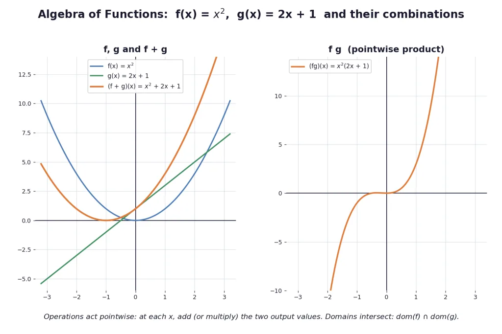
Key Point: These are operations on functions, producing functions. $(f + g)$ is itself a machine: feed it x, it feeds x to both f and g and adds the results.

[Board Important] When f and g have different domains, first restrict to the common ground: dom(f + g) = dom(f) $\cap$ dom(g), and the quotient additionally deletes the zeros of g.

Domain Bookkeeping — Where the New Function Lives

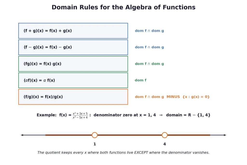
Each combined function exists only where every ingredient exists (and denominators are non-zero):

• $f + g$, $f - g$, $fg$ : domain = dom(f) $\cap$ dom(g)
• $\alpha f$ : domain = dom(f)
• $\frac{f}{g}$ : domain = dom(f) $\cap$ dom(g) $-$ {x : g(x) = 0}

The standard worked model

For $f(x) = x^2$ and $g(x) = 2x + 1$ (both with domain $\mathbb{R}$):

• $(f + g)(x) = x^2 + 2x + 1$
• $(f - g)(x) = x^2 - 2x - 1$
• $(fg)(x) = x^2(2x + 1) = 2x^3 + x^2$
• $\left(\frac{f}{g}\right)(x) = \frac{x^2}{2x + 1}$, valid for $x \neq -\frac{1}{2}$ (where g vanishes)

Notice $(f + g)(x) = (x + 1)^2$ — combining functions often produces recognisable new ones.

Rational functions revisited

A rational function is exactly a quotient $\frac{f}{g}$ of two polynomial functions, defined where the denominator is non-zero. Example: the domain of $\frac{x^2 + 3x + 5}{x^2 - 5x + 4}$ excludes the roots of $x^2 - 5x + 4 = (x - 1)(x - 4)$, giving domain $\mathbb{R} - \{1, 4\}$.

[JEE Tip] Domain questions on quotients are two mechanical steps: (1) intersect the ingredient domains; (2) solve g(x) = 0 and delete the roots. Write the answer in the form $\mathbb{R} - \{\ldots\}$ or as intervals — both are accepted, but interval form is safer when square roots also restrict the domain.

Solved Examples

Example 1. Let $f(x) = x^2$ and $g(x) = 2x + 1$. Find $(f + g)(x)$, $(f - g)(x)$, $(fg)(x)$ and $\left(\frac{f}{g}\right)(x)$.

Solution.

Step 1 — recall pointwise arithmetic. Each combination acts value-by-value: at input x, combine the numbers f(x) and g(x).

Step 2 — sum. $(f + g)(x) = x^2 + (2x + 1) = x^2 + 2x + 1$ — recognisably $(x + 1)^2$.

Step 3 — difference. $(f - g)(x) = x^2 - (2x + 1) = x^2 - 2x - 1$ (the minus hits BOTH terms).

Step 4 — product. $(fg)(x) = x^2(2x + 1) = 2x^3 + x^2$.

Step 5 — quotient with its exclusion. $\left(\frac{f}{g}\right)(x) = \frac{x^2}{2x + 1}$, valid only where $2x + 1 \neq 0$, i.e. $x \neq -\frac{1}{2}$.

Takeaway: state the excluded point with every quotient — it carries a mark, every single time.

Example 2. Let $f(x) = \sqrt{x}$ and $g(x) = x$ on the non-negative reals. Find $(f + g)(x)$, $(f - g)(x)$, $(fg)(x)$ and $\left(\frac{f}{g}\right)(x)$.

Solution.

Step 1 — sum and difference. $(f + g)(x) = \sqrt{x} + x$; $(f - g)(x) = \sqrt{x} - x$ — no simplification available, leave as is.

Step 2 — product via exponent rules. $(fg)(x) = x^{1/2} \cdot x^1 = x^{1/2 + 1} = x^{3/2}$.

Step 3 — quotient via exponent rules. $\left(\frac{f}{g}\right)(x) = \frac{x^{1/2}}{x^1} = x^{1/2 - 1} = x^{-1/2} = \frac{1}{\sqrt{x}}$, needing $x \neq 0$.

Step 4 — watch the domain shrink. f, g and their sum/product live on $[0, \infty)$, but the quotient silently drops 0: its domain is $(0, \infty)$.

Takeaway: handle root-times-power by adding/subtracting exponents, and track the quotient's shrunken domain explicitly.

Example 3. Let f, g : $\mathbb{R} \to \mathbb{R}$ be $f(x) = x + 1$ and $g(x) = 2x - 3$. Find $f + g$, $f - g$ and $\frac{f}{g}$.

Solution.

Step 1 — sum. $(f + g)(x) = (x + 1) + (2x - 3) = 3x - 2$.

Step 2 — difference, distributing the minus over ALL of g. $(f - g)(x) = (x + 1) - (2x - 3) = x + 1 - 2x + 3 = -x + 4$. (Note the $-(-3) = +3$.)

Step 3 — quotient with exclusion. $\left(\frac{f}{g}\right)(x) = \frac{x + 1}{2x - 3}$, valid where $2x - 3 \neq 0$, i.e. $x \neq \frac{3}{2}$.

Takeaway: the classic slip is losing the +3 when distributing the minus — bracket g fully before subtracting.

Example 4. Find the domain of $f(x) = \frac{x^2 + 2x + 1}{x^2 - 8x + 12}$.

Solution.

Step 1 — locate the only danger. A rational function fails exactly where its DENOMINATOR vanishes; the numerator never restricts.

Step 2 — factor the denominator. Product 12, sum $-8$: the numbers are $-2$ and $-6$, so $x^2 - 8x + 12 = (x - 2)(x - 6)$.

Step 3 — delete the zeros. $x = 2$ and $x = 6$ are excluded.

Step 4 — write the domain. $\mathbb{R} - \{2, 6\}$.

Takeaway: numerator roots (here $x = -1$) are harmless — only denominator zeros leave the domain.

Example 5. Find the domain of $f(x) = \frac{x^2 + 3x + 5}{x^2 - 5x + 4}$.

Solution.

Step 1 — factor the denominator. Product 4, sum $-5$: $x^2 - 5x + 4 = (x - 1)(x - 4)$.

Step 2 — delete its zeros. $x = 1$ and $x = 4$.

Step 3 — domain. $\mathbb{R} - \{1, 4\}$.

Takeaway: identical recipe every time — factor the denominator, delete its roots, keep everything else.

Example 6. Find the domain and range of $f(x) = \sqrt{x - 1}$.

Solution.

Step 1 — domain from the radicand. Need $x - 1 \geq 0$, i.e. $x \geq 1$: domain = $[1, \infty)$, the endpoint included since $\sqrt{0} = 0$.

Step 2 — range by tracking. As x sweeps $[1, \infty)$, the radicand $x - 1$ sweeps $[0, \infty)$, and the square root maps that onto $[0, \infty)$.

Step 3 — range. $[0, \infty)$.

Takeaway: for $\sqrt{\text{linear}}$, the domain starts at the zero of the inside and the range is always $[0, \infty)$.

Example 7. Find the domain and range of $f(x) = |x - 1|$.

Solution.

Step 1 — domain. The modulus accepts every real number: domain = $\mathbb{R}$.

Step 2 — range, lower end. $|x - 1| \geq 0$ always, and the value 0 IS attained — at x = 1, the corner of the V.

Step 3 — range, coverage. Any target $y > 0$ is hit by $x = 1 + y$: range = $[0, \infty)$.

Takeaway: shifting INSIDE the modulus moves the corner (to x = 1) but leaves the range untouched at $[0, \infty)$.

Example 8. Let $f = \left\{\left(x, \frac{x^2}{1 + x^2}\right) : x \in \mathbb{R}\right\}$. Determine the range of f.

Solution.

Step 1 — bound the outputs. Since $0 \leq x^2 < 1 + x^2$, dividing gives $0 \leq \frac{x^2}{1 + x^2} < 1$ — every output lies in $[0, 1)$.

Step 2 — determine WHICH values occur: solve for x in terms of y. Set $y = \frac{x^2}{1 + x^2}$. Then $y(1 + x^2) = x^2$, so $y = x^2(1 - y)$ and $x^2 = \frac{y}{1 - y}$.

Step 3 — solvability condition. A real x exists exactly when $\frac{y}{1 - y} \geq 0$, i.e. $0 \leq y < 1$ — precisely the interval from Step 1, all of it attained (y = 0 at x = 0).

Step 4 — the excluded endpoint. $y = 1$ would demand $x^2 = 1 + x^2$ — impossible. Range = $[0, 1)$.

Takeaway: \"solve for x in terms of y\" converts range-finding into a solvability question — the single most powerful range technique you will carry into Class 12 and JEE.

Example 9. If $f(x) = x^2$, find $\frac{f(1.1) - f(1)}{1.1 - 1}$.

Solution.

Step 1 — evaluate the function at both points. $f(1.1) = (1.1)^2 = 1.21$; $f(1) = 1$.

Step 2 — form the ratio. $\frac{1.21 - 1}{1.1 - 1} = \frac{0.21}{0.1} = 2.1$.

Step 3 — interpret. This is the average rate of change of $x^2$ between 1 and 1.1 — and as the second point slides toward 1, the ratio slides toward 2, the derivative of $x^2$ at 1.

Takeaway: the difference quotient is your first handshake with the derivative — Chapter 12 makes the limiting value precise.

Example 10. Let $f(x) = |x|$ and $g(x) = x$. Compute $(f + g)(x)$ and $(f - g)(x)$, and describe both.

Solution.

Step 1 — split $\mathbb{R}$ at the modulus boundary x = 0.

Step 2 — non-negative piece. For $x \geq 0$: $|x| = x$, so $(f + g)(x) = x + x = 2x$ and $(f - g)(x) = x - x = 0$.

Step 3 — negative piece. For $x < 0$: $|x| = -x$, so $(f + g)(x) = -x + x = 0$ and $(f - g)(x) = -x - x = -2x$.

Step 4 — describe. $f + g$: zero on the negatives, the line 2x on the positives. $f - g$: the mirror image — $-2x$ on the negatives, zero on the positives.

Takeaway: to combine piecewise functions, split the real line at every formula boundary and work each piece separately.

Example 11. With $f(x) = x^2$ and $g(x) = 2x + 1$, find $(3f)(x)$, $(-g)(x)$ and $(2f - 3g)(x)$, and evaluate $(2f - 3g)(2)$.

Solution.

Step 1 — scalar multiples. $(3f)(x) = 3x^2$; $(-g)(x) = -(2x + 1) = -2x - 1$.

Step 2 — the linear combination. $(2f - 3g)(x) = 2x^2 - 3(2x + 1) = 2x^2 - 6x - 3$.

Step 3 — evaluate at x = 2. $2(2^2) - 6(2) - 3 = 8 - 12 - 3 = -7$. Cross-check pointwise: $2f(2) - 3g(2) = 2(4) - 3(5) = 8 - 15 = -7$ ✓.

Takeaway: linear combinations of functions behave exactly like linear combinations of numbers, applied pointwise — and the two evaluation orders must agree.

Example 12. Find the domain of $\left(\frac{f}{g}\right)(x)$ where $f(x) = \sqrt{x}$ and $g(x) = x^2 - 4$.

Solution.

Step 1 — ingredient domains. dom(f) = $[0, \infty)$ (radicand $\geq 0$); dom(g) = $\mathbb{R}$.

Step 2 — intersect. $[0, \infty) \cap \mathbb{R} = [0, \infty)$.

Step 3 — delete the zeros of g. $x^2 - 4 = 0$ at $x = 2$ and $x = -2$; of these only $x = 2$ lies in $[0, \infty)$ — deleting $-2$ changes nothing.

Step 4 — write the domain. $[0, \infty) - \{2\} = [0, 2) \cup (2, \infty)$.

Takeaway: both rules fire together — the root restricts first, the quotient punches out surviving zeros; interval form displays the hole clearly.

Example 13. Let $f(x) = \sqrt{x - 1}$ and $g(x) = \sqrt{5 - x}$. Find the domain of $(f + g)(x) = \sqrt{x - 1} + \sqrt{5 - x}$.

Solution.

Step 1 — domain of each root. First: $x - 1 \geq 0 \Rightarrow x \geq 1$, i.e. $[1, \infty)$. Second: $5 - x \geq 0 \Rightarrow x \leq 5$, i.e. $(-\infty, 5]$.

Step 2 — the sum needs BOTH. Intersect: $[1, \infty) \cap (-\infty, 5] = [1, 5]$.

Step 3 — endpoint check. At x = 1: $\sqrt{0} + \sqrt{4}$ defined ✓; at x = 5: $\sqrt{4} + \sqrt{0}$ ✓ — both endpoints stay.

Takeaway: two one-sided conditions intersect to a closed interval — sketch both on a number line and read off the overlap.

Example 14. For $f(x) = x + 1$ and $g(x) = 2x - 3$, verify at x = 4 that $(fg)(4) = f(4)\,g(4)$ and compute $(fg)(x)$ in general.

Solution.

Step 1 — expand the general product. $(fg)(x) = (x + 1)(2x - 3) = 2x^2 - 3x + 2x - 3 = 2x^2 - x - 3$.

Step 2 — evaluate via the formula. $(fg)(4) = 2(16) - 4 - 3 = 32 - 7 = 25$.

Step 3 — evaluate pointwise. $f(4) = 5$ and $g(4) = 5$, so $f(4)g(4) = 25$ ✓ — the two routes agree.

Takeaway: \"multiply then substitute\" and \"substitute then multiply\" must match — a free self-check on any expansion.

Example 15. The function $f(x) = x + 10$ on $\mathbb{R}$ is a linear function. Describe its graph and state its domain and range; then do the same for $(\alpha f)$ with $\alpha = \frac{1}{2}$.

Solution.

Step 1 — anchor two points of f. $f(0) = 10$ and $f(-10) = 0$: the graph is the straight line of slope 1 through (0, 10) and ($-10$, 0).

Step 2 — domain and range of f. Defined everywhere: domain $\mathbb{R}$. Any target y is hit by $x = y - 10$: range $\mathbb{R}$.

Step 3 — the scalar multiple. $\left(\frac{1}{2}f\right)(x) = \frac{x + 10}{2} = \frac{x}{2} + 5$: slope $\frac{1}{2}$, y-intercept 5.

Step 4 — its domain and range. Still all of $\mathbb{R}$ for both — a non-zero scalar cannot shrink a line's range.

Takeaway: every linear function $mx + c$ with $m \neq 0$ has domain AND range $\mathbb{R}$; scalars tilt the line but never truncate it.