Axiomatic Probability and Equally Likely Outcomes

The Three Axioms

Earlier classes assigned probabilities by counting. The axiomatic approach (Kolmogorov) instead lays down rules that ANY probability must obey, and derives everything else from them.

Let $S$ be the sample space of a random experiment. Probability is a real-valued function $P$ whose domain is the collection of events of $S$ and whose range is $[0, 1]$, satisfying:

1. Axiom 1: $P(E) \geq 0$ for any event $E$;
2. Axiom 2: $P(S) = 1$;
3. Axiom 3: if $E$ and $F$ are mutually exclusive, then $P(E \cup F) = P(E) + P(F)$.

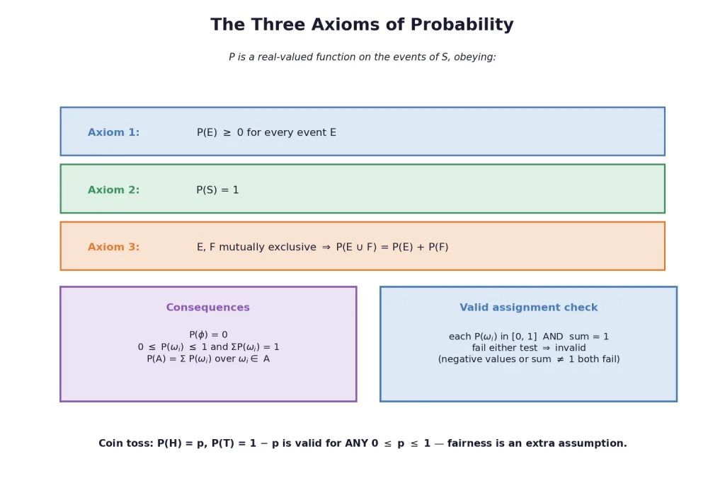
First consequence: $P(\phi) = 0$. Take $F = \phi$ in Axiom 3 ($E$ and $\phi$ are disjoint): $P(E \cup \phi) = P(E) + P(\phi)$, i.e. $P(E) = P(E) + P(\phi)$, forcing $P(\phi) = 0$.

For a finite sample space $S = \{\omega_1, \omega_2, \ldots, \omega_n\}$ the axioms boil down to three working rules:

• $0 \leq P(\omega_i) \leq 1$ for each outcome;
• $P(\omega_1) + P(\omega_2) + \cdots + P(\omega_n) = 1$;
• for any event $A$: $\;P(A) = \sum P(\omega_i)$ over all $\omega_i \in A$.

(For a singleton we write $P(\omega_i)$ instead of $P(\{\omega_i\})$.)

Many Valid Assignments

The axioms do NOT force fairness. For one coin toss, $P(H) = \frac{1}{2}, P(T) = \frac{1}{2}$ is valid — but so is $P(H) = \frac{1}{4}, P(T) = \frac{3}{4}$, and in general $P(H) = p$, $P(T) = 1 - p$ for any $0 \leq p \leq 1$. There are infinitely many valid assignments; the axioms only police non-negativity and total 1.

Checking validity is a two-part test: every $P(\omega_i)$ must lie in $[0, 1]$, and the sum must be exactly 1. Fail either part and the assignment is invalid — a negative entry sinks it even if the sum is 1, and a sum of 2.1 sinks it even if every entry looks innocent.

Computing an event's probability from an assignment. With $S = \{HH, HT, TH, TT\}$ and the (unequal!) assignment $P(HH) = \frac{1}{4}$, $P(HT) = \frac{1}{7}$, $P(TH) = \frac{2}{7}$, $P(TT) = \frac{9}{28}$, the event $E$ = 'both tosses give the same result' $= \{HH, TT\}$ has

$$P(E) = P(HH) + P(TT) = \frac{1}{4} + \frac{9}{28} = \frac{7 + 9}{28} = \frac{16}{28} = \frac{4}{7}.$$

Add the sample-point probabilities — that is the whole method.

Equally Likely Outcomes

When all $n$ outcomes have the same chance $p$, the sum condition gives $np = 1$, so $p = \frac{1}{n}$. For an event $E$ with $n(E) = m$ favourable outcomes,

$$P(E) = \frac{m}{n} = \frac{\text{number of outcomes favourable to } E}{\text{total possible outcomes}} = \frac{n(E)}{n(S)}.$$

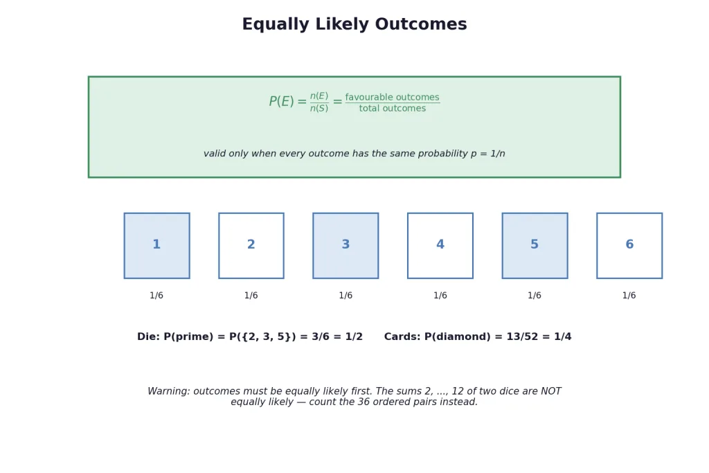
This is the classical formula from earlier classes — now derived as a theorem, valid only under equal likelihood. A fair die gives $P(\text{prime}) = \frac{3}{6} = \frac{1}{2}$; a shuffled deck gives $P(\text{diamond}) = \frac{13}{52} = \frac{1}{4}$.

Standing convention: from here on, examples and exercises assume equally likely outcomes unless stated otherwise.

Warning. Choose a sample space whose outcomes really are equally likely. For two dice, the eleven sums $2, 3, \ldots, 12$ are NOT equally likely; the 36 ordered pairs are — always count pairs, then group them by sum.

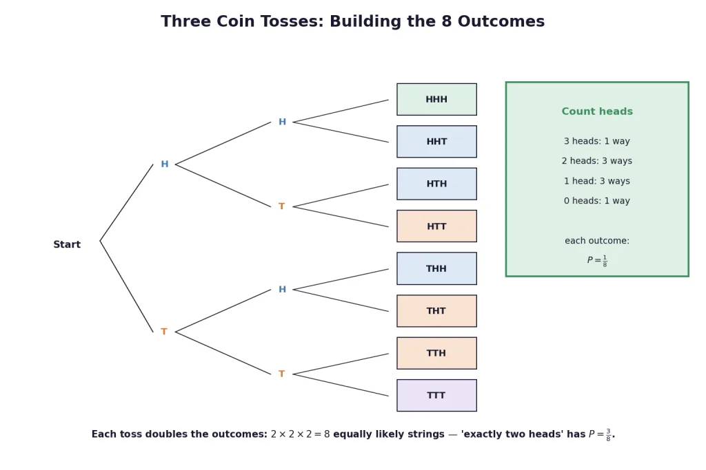
The tree shows why repeated tosses multiply outcomes: each stage doubles the count, and every full path is equally likely.

Solved Examples

Example 1. $S = \{\omega_1, \ldots, \omega_6\}$. Which assignments of probabilities are valid?

	$\omega_1$	$\omega_2$	$\omega_3$	$\omega_4$	$\omega_5$	$\omega_6$
(a)	$\frac{1}{6}$	$\frac{1}{6}$	$\frac{1}{6}$	$\frac{1}{6}$	$\frac{1}{6}$	$\frac{1}{6}$
(b)	$1$	$0$	$0$	$0$	$0$	$0$
(c)	$\frac{1}{8}$	$\frac{2}{3}$	$\frac{1}{3}$	$\frac{1}{3}$	$-\frac{1}{4}$	$-\frac{1}{3}$
(d)	$\frac{1}{12}$	$\frac{1}{12}$	$\frac{1}{6}$	$\frac{1}{6}$	$\frac{1}{6}$	$\frac{3}{2}$
(e)	$0.1$	$0.2$	$0.3$	$0.4$	$0.5$	$0.6$

Solution. Apply the two-part test to each row: every entry must lie in $[0, 1]$, and the six entries must add to exactly 1.

(a) Entries: each $\frac{1}{6} \in [0,1]$ ✓. Sum: $6 \times \frac{1}{6} = 1$ ✓. Valid — the fair-die assignment.

(b) Entries: 1 and 0 are both allowed values ✓. Sum: $1 + 0 + 0 + 0 + 0 + 0 = 1$ ✓. Valid — extreme, but legal: outcome $\omega_1$ is certain.

(c) $P(\omega_5) = -\frac{1}{4}$ and $P(\omega_6) = -\frac{1}{3}$ are negative, violating Axiom 1. Invalid (no need to even check the sum — one failed test is enough).

(d) $P(\omega_6) = \frac{3}{2} > 1$, impossible for a probability. Invalid.

(e) Entries all lie in $[0,1]$, but the sum is $0.1 + 0.2 + 0.3 + 0.4 + 0.5 + 0.6 = 2.1 \neq 1$. Invalid.

---

Example 2. One card is drawn from a well-shuffled deck of 52. Find the probability the card is (i) a diamond (ii) not an ace (iii) a black card (iv) not a diamond (v) not a black card.

Solution.

Step 1 — set up. A well-shuffled deck makes all 52 cards equally likely, so each part is a count divided by 52.

Step 2 — (i). The deck has 13 diamonds: $P(\text{diamond}) = \frac{13}{52} = \frac{1}{4}$.

Step 3 — (ii) via the complement. There are 4 aces, so $P(\text{ace}) = \frac{4}{52} = \frac{1}{13}$, and $P(\text{not ace}) = 1 - \frac{1}{13} = \frac{12}{13}$ — one subtraction instead of counting 48 cards.

Step 4 — (iii). Black cards are the clubs and spades: $13 + 13 = 26$, so $P(\text{black}) = \frac{26}{52} = \frac{1}{2}$.

Step 5 — (iv) and (v), complements again. $P(\text{not diamond}) = 1 - \frac{1}{4} = \frac{3}{4}$; $P(\text{not black}) = 1 - \frac{1}{2} = \frac{1}{2}$.

---

Example 3. A bag contains 9 discs: 4 red, 3 blue, 2 yellow. One disc is drawn at random. Find the probability it is (i) red (ii) yellow (iii) blue (iv) not blue (v) either red or blue.

Solution.

Step 1 — set up. 'At random' from $4 + 3 + 2 = 9$ identical-feeling discs means 9 equally likely outcomes.

Step 2 — direct counts. (i) $P(\text{red}) = \frac{4}{9}$. (ii) $P(\text{yellow}) = \frac{2}{9}$. (iii) $P(\text{blue}) = \frac{3}{9} = \frac{1}{3}$.

Step 3 — (iv) complement. $P(\text{not blue}) = 1 - P(\text{blue}) = 1 - \frac{1}{3} = \frac{2}{3}$.

Step 4 — (v) disjoint addition. A single disc cannot be red and blue at once, so the events are mutually exclusive and probabilities add: $P(\text{red or blue}) = \frac{4}{9} + \frac{1}{3} = \frac{4}{9} + \frac{3}{9} = \frac{7}{9}$. Check against direct counting: $4 + 3 = 7$ favourable discs of 9. ✓

---

Example 4. Which of the following cannot be a valid assignment for $S = \{\omega_1, \ldots, \omega_7\}$?

(a) $0.1, 0.01, 0.05, 0.03, 0.01, 0.2, 0.6$ (b) each $\frac{1}{7}$ (c) $0.1, 0.2, 0.3, 0.4, 0.5, 0.6, 0.7$ (d) $-0.1, 0.2, 0.3, 0.4, -0.2, 0.1, 0.3$ (e) $\frac{1}{14}, \frac{2}{14}, \frac{3}{14}, \frac{4}{14}, \frac{5}{14}, \frac{6}{14}, \frac{15}{14}$

Solution. Same two-part test, seven outcomes now.

(a) Sum: $0.1 + 0.01 + 0.05 + 0.03 + 0.01 + 0.2 + 0.6 = 1.00$ ✓, all entries in $[0,1]$ ✓ — valid.

(b) Sum: $7 \times \frac{1}{7} = 1$ ✓ — valid (equally likely case).

(c) Sum: $0.1 + 0.2 + \cdots + 0.7 = 2.8 \neq 1$ — cannot be valid.

(d) Two entries ($-0.1$ and $-0.2$) are negative — cannot be valid, regardless of the sum.

(e) $\frac{15}{14} > 1$ breaks the range test (and the sum $\frac{1+2+3+4+5+6+15}{14} = \frac{36}{14} \neq 1$ breaks the total too) — cannot be valid.

---

Example 5. A coin is tossed twice. What is the probability that atleast one tail occurs?

Solution.

Step 1 — sample space. Two tosses: $S = \{HH, HT, TH, TT\}$, four equally likely outcomes.

Step 2 — spot the complement. 'Atleast one tail' fails only for the single outcome $HH$.

Step 3 — compute. $P(\text{atleast one tail}) = 1 - P(HH) = 1 - \frac{1}{4} = \frac{3}{4}$. Direct check: the favourable outcomes $\{HT, TH, TT\}$ are 3 of 4. ✓

---

Example 6. A die is thrown. Find the probability of: (i) a prime number (ii) a number $\geq 3$ (iii) a number $\leq 1$ (iv) a number more than 6 (v) a number less than 6.

Solution. Each part: list the favourable faces, count, divide by 6.

(i) Primes: $\{2, 3, 5\}$ — three faces → $\frac{3}{6} = \frac{1}{2}$.

(ii) Atleast 3: $\{3, 4, 5, 6\}$ — four faces → $\frac{4}{6} = \frac{2}{3}$.

(iii) Atmost 1: only $\{1\}$ → $\frac{1}{6}$.

(iv) More than 6: no face qualifies — the impossible event → $P = 0$.

(v) Less than 6: $\{1, 2, 3, 4, 5\}$ → $\frac{5}{6}$; equivalently $1 - P(6) = 1 - \frac{1}{6}$.

---

Example 7. A fair coin with 1 on one face and 6 on the other, and a fair die, are both tossed. Find the probability that the sum is (i) 3 (ii) 12.

Solution.

Step 1 — build the sample space. Record (coin, die): $2 \times 6 = 12$ equally likely pairs.

Step 2 — (i) hunt for sum 3. Coin 1 needs die $3 - 1 = 2$: the pair $(1, 2)$ ✓. Coin 6 needs die $3 - 6 = -3$: impossible. Exactly one favourable pair → $P = \frac{1}{12}$.

Step 3 — (ii) hunt for sum 12. Coin 1 needs die 11: impossible. Coin 6 needs die 6: the pair $(6, 6)$ ✓. Again one pair → $P = \frac{1}{12}$.

---

Example 8. A fair coin is tossed four times; a person wins Re 1 per head and loses Rs 1.50 per tail. Find the possible amounts and their probabilities.

Solution.

Step 1 — reduce the money to the head-count. With $k$ heads there are $4 - k$ tails, so the amount is $k(1) - (4 - k)(1.50) = 2.5k - 6$ rupees. Different $k$ give different amounts, so five values of $k$ (0 to 4) give five amounts.

Step 2 — probability of each head-count. Of the $2^4 = 16$ equally likely toss-strings, exactly $\binom{4}{k}$ have $k$ heads.

Step 3 — tabulate.

Heads $k$	Amount $2.5k - 6$ (Rs)	Strings $\binom{4}{k}$	Probability
4	$4.00$	1	$\frac{1}{16}$
3	$1.50$	4	$\frac{4}{16} = \frac{1}{4}$
2	$-1.00$	6	$\frac{6}{16} = \frac{3}{8}$
1	$-3.50$	4	$\frac{4}{16} = \frac{1}{4}$
0	$-6.00$	1	$\frac{1}{16}$

Step 4 — verify. $\frac{1 + 4 + 6 + 4 + 1}{16} = \frac{16}{16} = 1$ ✓.

---

Example 9. Three coins are tossed once. Find the probability of (i) 3 heads (ii) 2 heads (iii) atleast 2 heads (iv) atmost 2 heads (v) no head (vi) 3 tails (vii) exactly two tails (viii) no tail (ix) atmost two tails.

Solution.

Step 1 — sample space. $2^3 = 8$ equally likely strings: $HHH, HHT, HTH, THH, HTT, THT, TTH, TTT$.

Step 2 — single-count parts. (i) 3 heads: only $HHH$ → $\frac{1}{8}$. (v) no head: only $TTT$ → $\frac{1}{8}$. (vi) 3 tails is the same event as no head → $\frac{1}{8}$. (viii) no tail is the same as 3 heads → $\frac{1}{8}$.

Step 3 — exactly-two parts. (ii) exactly 2 heads: choose which two tosses are heads, $\binom{3}{2} = 3$ strings ($HHT, HTH, THH$) → $\frac{3}{8}$. (vii) exactly two tails: symmetric, $\{HTT, THT, TTH\}$ → $\frac{3}{8}$.

Step 4 — cumulative parts. (iii) atleast 2 heads $=$ exactly 2 or exactly 3: $\frac{3}{8} + \frac{1}{8} = \frac{1}{2}$. (iv) atmost 2 heads is the complement of '3 heads': $1 - \frac{1}{8} = \frac{7}{8}$. (ix) atmost two tails is the complement of '3 tails': $1 - \frac{1}{8} = \frac{7}{8}$.

---

Example 10. (a) If $\frac{2}{11}$ is the probability of an event $A$, find $P(\text{not } A)$. (b) A letter is chosen at random from 'ASSASSINATION'. Find the probability it is (i) a vowel (ii) a consonant.

Solution.

(a) Step 1: the complement rule gives $P(A') = 1 - P(A)$. Step 2: $P(A') = 1 - \frac{2}{11} = \frac{9}{11}$.

(b) Step 1 — inventory the word. ASSASSINATION spells A-S-S-A-S-S-I-N-A-T-I-O-N: 13 letters, with A × 3, S × 4, I × 2, N × 2, T × 1, O × 1 (check: $3+4+2+2+1+1 = 13$ ✓).

Step 2 — count vowels and consonants. Vowels (A, I, O): $3 + 2 + 1 = 6$. Consonants (S, N, T): $4 + 2 + 1 = 7$.

Step 3 — divide. Each of the 13 letter-positions is equally likely: (i) $P(\text{vowel}) = \frac{6}{13}$; (ii) $P(\text{consonant}) = \frac{7}{13}$. Check: $\frac{6}{13} + \frac{7}{13} = 1$ ✓.

---

Example 11. In a lottery a person chooses six different natural numbers at random from 1 to 20; he wins if they match the six fixed by the committee. Find the probability of winning.

Solution.

Step 1 — decide: order or no order? The prize depends only on WHICH six numbers are chosen, not the order of choosing — so outcomes are 6-element subsets.

Step 2 — count the sample space. Number of 6-subsets of $\{1, \ldots, 20\}$: $\binom{20}{6} = \frac{20 \times 19 \times 18 \times 17 \times 16 \times 15}{6!} = 38760$, all equally likely.

Step 3 — count favourable and divide. Exactly one subset matches the committee's choice: $P(\text{win}) = \frac{1}{38760}$.