JEE Corner — Statistics for JEE Main and Advanced

Linear Transformations and the Coefficient of Variation

The textbook proves the two halves separately; JEE tests them combined.

Key Point (Linear transformation): if $y_i = ax_i + b$, then

$$\bar{y} = a\bar{x} + b \qquad \sigma_y = |a|\,\sigma_x \qquad \sigma_y^2 = a^2\sigma_x^2$$

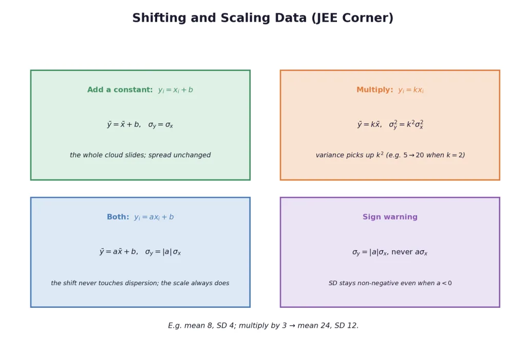
The shift $b$ moves the centre and never touches the spread; the scale $a$ stretches both — and the SD takes $|a|$, never a negative value. This one law answers a whole family of JEE one-liners, including the step-deviation method itself (which is just $y = \frac{x - A}{h}$ run backwards).

The coefficient of variation — beyond the rationalised syllabus, but JEE still asks it:

Key Point (C.V.):

$$\mathrm{C.V.} = \frac{\sigma}{\bar{x}} \times 100 \qquad (\bar{x} \ne 0)$$

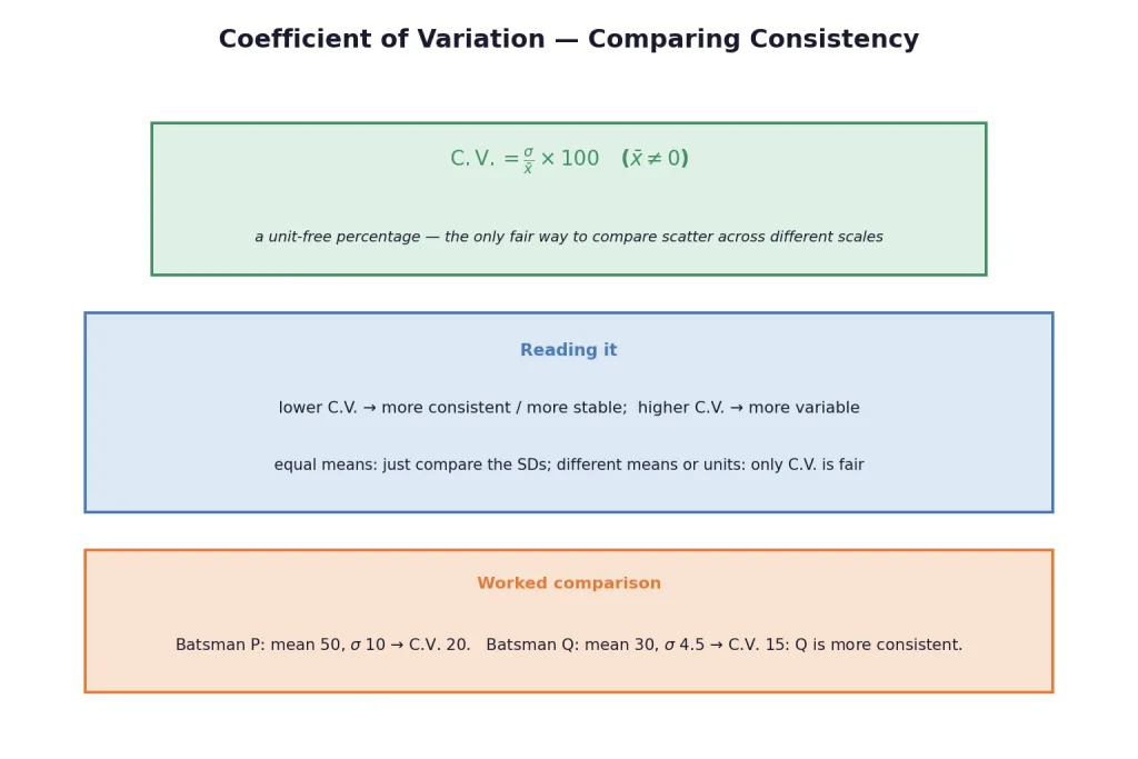
A unit-free percentage: it lets you compare scatter across different scales or units. Lower C.V. = more consistent. When two series share the same mean, comparing SDs is enough; otherwise only C.V. is fair. Example: batsman P (mean 50, $\sigma$ 10, C.V. 20) vs batsman Q (mean 30, $\sigma$ 4.5, C.V. 15) — Q is the more consistent scorer despite the lower average.

The $\sum x^2$ Identity and Combined Groups

1. The computing identity, formalised.

$$\sigma^2 = \frac{\sum x_i^2}{n} - \bar{x}^2 \quad\Longleftrightarrow\quad \sum x_i^2 = n\left(\sigma^2 + \bar{x}^2\right)$$

Every missing-observation and corrected-statistics problem is this identity plus bookkeeping. A free by-product: since $\sigma^2 \ge 0$,

$$\frac{\sum x_i^2}{n} \ge \left(\frac{\sum x_i}{n}\right)^2$$

— the mean of squares always dominates the square of the mean, with equality only for constant data.

2. Combined mean and variance of two groups. Groups of sizes $n_1, n_2$ with means $\bar{x}_1, \bar{x}_2$ and variances $\sigma_1^2, \sigma_2^2$:

Key Point (Combined statistics):

$$\bar{x} = \frac{n_1\bar{x}_1 + n_2\bar{x}_2}{n_1 + n_2} \qquad \sigma^2 = \frac{n_1(\sigma_1^2 + d_1^2) + n_2(\sigma_2^2 + d_2^2)}{n_1 + n_2}$$

where $d_i = \bar{x}_i - \bar{x}$ measures how far each group's mean sits from the combined mean. When the group means coincide ($d_1 = d_2 = 0$), the combined variance is simply the weighted average of the variances; when they differ, the between-group spread adds on top.

[JEE Tip] Almost every statistics question in JEE Main resolves into three tools: the $\sum x^2$ identity, the linear-transformation law, and (occasionally) combined groups. Translate the words into $\sum x_i$ and $\sum x_i^2$ first — the rest is arithmetic.

JEE-Style Solved Examples

Example 1: C.V. comparison

Batsman P: mean 50, $\sigma = 10$. Batsman Q: mean 30, $\sigma = 4.5$. Who is more consistent?

Solution:

Step 1 — Compute both C.V.s. C.V.(P) $= \frac{10}{50} \times 100 = 20$; C.V.(Q) $= \frac{4.5}{30} \times 100 = 15$.

Step 2 — Compare. Lower C.V. = more consistent: Q wins, despite the lower average.

Takeaway: With different means, raw SDs are unfair — only the RELATIVE scatter (C.V.) compares consistency across scales.

Example 2: Mean from C.V.

A series has C.V. 40 and $\sigma = 8$. Find the mean.

Solution:

Step 1 — Write the definition. $40 = \frac{8}{\bar{x}} \times 100$.

Step 2 — Solve. $\bar{x} = \frac{800}{40} = 20$.

Takeaway: The C.V. definition holds three quantities — given any two, one division recovers the third.

Example 3: Full linear transformation

Data has mean 10 and SD 2. Compute the mean and SD of $y = 3x + 5$.

Solution:

Step 1 — Mean takes both. $\bar{y} = 3(10) + 5 = 35$.

Step 2 — SD takes only the scale. $\sigma_y = |3| \times 2 = 6$.

Takeaway: The mean obeys the whole transformation; the SD hears only the multiplier — never add the shift to a spread.

Example 4: A negative scale

Data has SD 2. Find the SD of $y = -4x + 7$.

Solution:

Step 1 — Discard the shift. The 7 cannot touch the SD.

Step 2 — Absolute value of the scale. $\sigma_y = |-4| \times 2 = 8$.

Takeaway: A negative multiplier flips the data's ORDER but not its spread — the modulus in $|a|\sigma$ is doing real work.

Example 5: Combined mean

Section A (30 students) averages 60 marks; section B (20 students) averages 55. Find the combined mean.

Solution:

Step 1 — Weight by group sizes. $\bar{x} = \frac{30(60) + 20(55)}{30 + 20}$.

Step 2 — Compute. $= \frac{1800 + 1100}{50} = 58$.

Takeaway: The combined mean is size-weighted — it sits closer to the LARGER group's mean (58 is nearer 60 than 55).

Example 6: Combined variance

Group 1: $n_1 = 100$, mean 15, variance 9. Group 2: $n_2 = 150$, mean 20, variance 16. Find the combined variance.

Solution:

Step 1 — Combined mean. $\bar{x} = \frac{1500 + 3000}{250} = 18$; hence $d_1 = 15 - 18 = -3$, $d_2 = 20 - 18 = 2$.

Step 2 — The formula. $\sigma^2 = \frac{100(9 + 9) + 150(16 + 4)}{250}$.

Step 3 — Compute. $= \frac{1800 + 3000}{250} = 19.2$.

Takeaway: Combined spread = within-group variances PLUS between-group separation ($d_i^2$) — 19.2 exceeds both 9 and 16's weighted average because the means differ.

Example 7: The identity as an inequality

Ten observations satisfy $\sum x_i = 30$. What is the least possible value of $\sum x_i^2$?

Solution:

Step 1 — Use $\sigma^2 \ge 0$. $\frac{\sum x_i^2}{10} \ge \left(\frac{30}{10}\right)^2 = 9$.

Step 2 — Conclude. $\sum x_i^2 \ge 90$.

Step 3 — When is it attained? Equality means $\sigma^2 = 0$: every observation equals 3.

Takeaway: "Variance is non-negative" doubles as an optimisation tool — the minimum of $\sum x_i^2$ under a fixed sum is at constant data.

Example 8: Sums from statistics

100 observations have mean 50 and SD 4. Find $\sum x_i$ and $\sum x_i^2$.

Solution:

Step 1 — First sum. $\sum x_i = 100 \times 50 = 5000$.

Step 2 — Second sum. $\sum x_i^2 = n(\sigma^2 + \bar{x}^2) = 100(16 + 2500) = 251600$.

Takeaway: $(\bar{x}, \sigma) \to (\sum x_i, \sum x_i^2)$ is the standard opening move of every corrected-statistics problem.

Example 9: Undoing a coding

After the coding $y = \frac{x - 25}{10}$, a data set shows $\bar{y} = 2$ and $\sigma_y = 1$. Find the original mean and SD.

Solution:

Step 1 — Invert the coding. $x = 10y + 25$.

Step 2 — Mean. $\bar{x} = 10(2) + 25 = 45$.

Step 3 — SD. $\sigma_x = 10 \times 1 = 10$.

Takeaway: This is the step-deviation method run backwards — coding and decoding are the same law read in two directions.

Example 10: Equal means, combined variance

Two groups of sizes 40 and 60 both have mean 20, with variances 4 and 9. Find the combined variance.

Solution:

Step 1 — The $d_i$ vanish. Both group means equal the combined mean: $d_1 = d_2 = 0$.

Step 2 — Weighted average of variances. $\sigma^2 = \frac{40(4) + 60(9)}{100} = \frac{700}{100} = 7$.

Takeaway: Equal means collapse the combined-variance formula to a plain weighted average — the $d_i^2$ terms exist only for separated groups.

Example 11: C.V. across units

Heights: mean 160 cm, $\sigma$ 8 cm. Weights: mean 60 kg, $\sigma$ 4.5 kg. Which varies more?

Solution:

Step 1 — C.V. of each. Heights: $\frac{8}{160} \times 100 = 5$; weights: $\frac{4.5}{60} \times 100 = 7.5$.

Step 2 — Compare. Weights are relatively more variable.

Step 3 — Why C.V. was forced. Comparing 8 cm against 4.5 kg directly is meaningless — different units; the C.V.'s unit-free percentage makes them commensurable.

Takeaway: Cross-unit comparisons are C.V.'s home ground — that is exactly what dividing by the mean buys.

Example 12: Transformation meets the identity

Data with $n = 5$ has $\sum x_i = 20$ and $\sum x_i^2 = 90$. Find the variance of $2x_i + 1$.

Solution:

Step 1 — Variance of $x$. $\sigma_x^2 = \frac{90}{5} - \left(\frac{20}{5}\right)^2 = 18 - 16 = 2$.

Step 2 — Transform. The $+1$ is invisible; the 2 squares: $\sigma^2 = 4 \times 2 = 8$.

Takeaway: JEE chains the two tools — identity first for $\sigma_x^2$, then the transformation law; the chain is worth rehearsing until automatic.