Range and Mean Deviation

Why Averages Are Not Enough

Two batsmen can both average 51 — one scoring 0, 27, 56, 117 and beyond, the other 46 to 60 every time. The mean hides the difference; what separates them is dispersion (scatter).

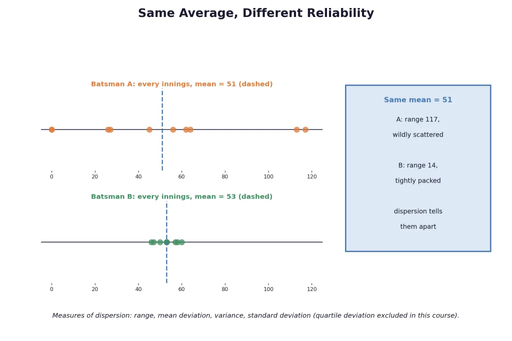
Key Point (Range): Range $=$ Maximum value $-$ Minimum value — the quickest measure of scatter. Batsman A: $117 - 0 = 117$; batsman B: $60 - 46 = 14$.

The range is rough: it uses only two observations and says nothing about how values cluster around a centre. For that we look at deviations $x_i - a$ from a central value $a$. But plain averaging fails — deviations about the mean sum to exactly zero. The fix: drop the signs.

Key Point (Mean deviation): about a central value $a$ (mean or median),

$$\mathrm{M.D.}(a) = \frac{1}{n}\sum_{i=1}^{n} |x_i - a|$$

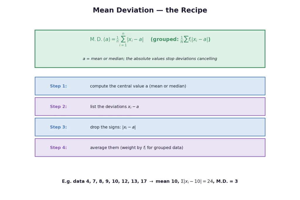
The four steps: find $a$; list deviations; take absolute values; average. For the data $4, 7, 8, 9, 10, 12, 13, 17$: mean 10, absolute deviations sum to 24, so $\mathrm{M.D.}(\bar{x}) = 3$.

Mean Deviation for Grouped Data

For a discrete frequency distribution ($x_i$ with frequencies $f_i$, $N = \sum f_i$):

$$\mathrm{M.D.}(\bar{x}) = \frac{1}{N}\sum f_i|x_i - \bar{x}|, \qquad \bar{x} = \frac{1}{N}\sum f_ix_i$$

About the median: arrange values in order, locate where the cumulative frequency first reaches $\frac{N}{2}$, and use that value as the median.

For a continuous frequency distribution, classes are represented by their midpoints, and the median comes from the grouped-median formula:

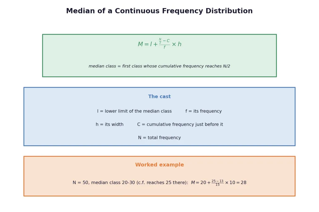
Key Point (Grouped median):

$$M = l + \frac{\frac{N}{2} - C}{f} \times h$$

where $l$, $f$, $h$ are the lower limit, frequency and width of the median class (the first class whose cumulative frequency reaches $\frac{N}{2}$), and $C$ is the cumulative frequency just before it. For example: $N = 50$, median class $20$-$30$, $M = 20 + \frac{25 - 13}{15} \times 10 = 28$, and $\mathrm{M.D.}(M) = \frac{508}{50} = 10.16$.

Limitations: mean deviation ignores signs, resists further algebra, and the median version is unreliable for highly variable data. These weaknesses motivate the standard deviation of the next section.

[Board Tip] For gapped classes like 16-20, 21-25 (and so on), first make them continuous (15.5-20.5, 20.5-25.5, and so on) by shifting each boundary half a unit — a step examiners check.

Solved Examples

Example 1: M.D. about the mean, ungrouped

Find the mean deviation about the mean: (i) $4, 7, 8, 9, 10, 12, 13, 17$; (ii) $38, 70, 48, 40, 42, 55, 63, 46, 54, 44$.

Solution:

Step 1 — (i) Mean first. $\bar{x} = \frac{80}{8} = 10$.

Step 2 — (i) Absolute deviations. $6, 3, 2, 1, 0, 2, 3, 7$ — sum 24.

Step 3 — (i) Average. M.D. $= \frac{24}{8} = 3$.

Step 4 — (ii) Same recipe. $\bar{x} = \frac{500}{10} = 50$; $\sum|x_i - 50| = 12+20+2+10+8+5+13+4+4+6 = 84$: M.D. $= 8.4$.

Takeaway: Mean, deviations, drop signs, average — four steps, and the zero-sum trap of raw deviations never appears.

Example 2: M.D. about the median

Find the mean deviation about the median for $13, 17, 16, 14, 11, 13, 10, 16, 11, 18, 12, 17$.

Solution:

Step 1 — Sort and locate the middle. Sorted: $10, 11, 11, 12, 13, 13, 14, 16, 16, 17, 17, 18$; with $n = 12$, the median is the average of the 6th and 7th values: $\frac{13 + 14}{2} = 13.5$.

Step 2 — Absolute deviations. They sum to 28.

Step 3 — Average. M.D. $= \frac{28}{12} \approx 2.33$.

Takeaway: For an even $n$ the median is the average of the two middle values — sort FIRST, then count in.

Example 3: Another median case

Find the mean deviation about the median for $36, 72, 46, 42, 60, 45, 53, 46, 51, 49$.

Solution:

Step 1 — Sort. $36, 42, 45, 46, 46, 49, 51, 53, 60, 72$: median $= \frac{46 + 49}{2} = 47.5$.

Step 2 — Deviations. $11.5 + 5.5 + 2.5 + 1.5 + 1.5 + 1.5 + 3.5 + 5.5 + 12.5 + 24.5 = 70$.

Step 3 — Average. M.D. $= \frac{70}{10} = 7$.

Takeaway: One outlier (72) inflates deviations about ANY centre — but the median itself stayed put; that robustness is its selling point.

Example 4: Discrete frequency data, about the mean

(i) $x_i$: 5, 10, 15, 20, 25 with $f_i$: 7, 4, 6, 3, 5. (ii) $x_i$: 10, 30, 50, 70, 90 with $f_i$: 4, 24, 28, 16, 8.

Solution:

Step 1 — (i) Weighted mean. $N = 25$, $\sum f_ix_i = 350$: $\bar{x} = 14$.

Step 2 — (i) Weighted deviations. $\sum f_i|x_i - 14| = 63 + 16 + 6 + 18 + 55 = 158$: M.D. $= \frac{158}{25} = 6.32$.

Step 3 — (ii) Same. $N = 80$, $\sum f_ix_i = 4000$: $\bar{x} = 50$; $\sum f_i|x_i - 50| = 160 + 480 + 0 + 320 + 320 = 1280$: M.D. $= 16$.

Takeaway: Frequencies weight everything — the formula is the ungrouped one with $f_i$ riding along and $N$ replacing $n$.

Example 5: Discrete frequency data, about the median

(i) $x_i$: 5, 7, 9, 10, 12, 15 with $f_i$: 8, 6, 2, 2, 2, 6. (ii) $x_i$: 15, 21, 27, 30, 35 with $f_i$: 3, 5, 6, 7, 8.

Solution:

Step 1 — (i) Median by cumulative frequency. $N = 26$, $\frac{N}{2} = 13$; cumulative counts run $8, 14, \ldots$ — the 13th observation sits at $x = 7$: median 7.

Step 2 — (i) Weighted deviations. $\sum f_i|x_i - 7| = 16 + 0 + 4 + 6 + 10 + 48 = 84$: M.D. $= \frac{84}{26} \approx 3.23$.

Step 3 — (ii) Same. $N = 29$; cumulative $3, 8, 14, 21, 29$ — the 15th observation is at $x = 30$: median 30; $\sum f_i|x_i - 30| = 45 + 45 + 18 + 0 + 40 = 148$: M.D. $= \frac{148}{29} \approx 5.1$.

Takeaway: The median of frequency data is found by cumulative counting — find where the running total first reaches $\frac{N}{2}$.

Example 6: Continuous classes, about the mean

Income per day (Rs): classes 0-100 up to 700-800 with frequencies 4, 8, 9, 10, 7, 5, 4, 3. Find the M.D. about the mean.

Solution:

Step 1 — Represent classes by midpoints. $x_i = 50, 150, \ldots, 750$; $N = 50$.

Step 2 — Mean. $\sum f_ix_i = 17900$: $\bar{x} = 358$.

Step 3 — Weighted absolute deviations. $\sum f_i|x_i - 358| = 1232 + 1664 + 972 + 80 + 644 + 960 + 1168 + 1176 = 7896$: M.D. $= \frac{7896}{50} = 157.92$.

Takeaway: For continuous data every computation runs on midpoints — one substitution converts the problem to the discrete case.

Example 7: Heights of boys

Heights (cm): 95-105 up to 145-155 with frequencies 9, 13, 26, 30, 12, 10. Find the M.D. about the mean.

Solution:

Step 1 — Midpoints. $100, 110, 120, 130, 140, 150$; $N = 100$.

Step 2 — Mean. $\sum f_ix_i = 12530$: $\bar{x} = 125.3$.

Step 3 — Deviations. $\sum f_i|x_i - 125.3| = 227.7 + 198.9 + 137.8 + 141 + 176.4 + 247 = 1128.8$: M.D. $\approx 11.29$.

Takeaway: A decimal mean is no obstacle — carry it through the deviation column and round only at the end.

Example 8: M.D. about the grouped median

Marks: classes 0-10 up to 50-60 with frequencies 6, 8, 14, 16, 4, 2. Find the M.D. about the median.

Solution:

Step 1 — Find the median class. $N = 50$, $\frac{N}{2} = 25$; cumulative frequencies $6, 14, 28, \ldots$ — the class 20-30 is where the running total first reaches 25.

Step 2 — Apply the grouped-median formula. $M = 20 + \frac{25 - 14}{14} \times 10 = 20 + \frac{110}{14} \approx 27.86$.

Step 3 — Weighted deviations from $M$. With midpoints $5, 15, \ldots, 55$: $\sum f_i|x_i - M| \approx 517.14$: M.D. $\approx \frac{517.14}{50} = 10.34$.

Takeaway: $l$, $f$, $h$ all belong to the median class; $C$ is the count BEFORE it — label the four numbers before touching the formula.

Example 9: Make the classes continuous first

Ages of 100 persons: 16-20, 21-25 and so on up to 51-55 with frequencies 5, 6, 12, 14, 26, 12, 16, 9. Find the M.D. about the median.

Solution:

Step 1 — Close the gaps. Shift boundaries half a unit: $15.5$-$20.5$, $20.5$-$25.5$, and so on.

Step 2 — Median class. Cumulative frequencies $5, 11, 23, 37, 63, \ldots$: the class $35.5$-$40.5$ first reaches 50. $M = 35.5 + \frac{50 - 37}{26} \times 5 = 35.5 + 2.5 = 38$.

Step 3 — Deviations. Midpoints $18, 23, \ldots, 53$: $\sum f_i|x_i - 38| = 100 + 90 + 120 + 70 + 0 + 60 + 160 + 135 = 735$: M.D. $= 7.35$.

Takeaway: Gapped classes MUST be made continuous before the median formula — the half-unit shift is the step examiners check first.

Example 10: A range drill

Find the range of both batsmen's scores: A: $0, 27, 56, 64, 0, 26, 117, 113, 62, 45$; B: $46, 47, 50, 53, 53, 53, 58, 60, 57, 53$.

Solution:

Step 1 — Extremes. A: max 117, min 0. B: max 60, min 46.

Step 2 — Ranges. A: $117 - 0 = 117$; B: $60 - 46 = 14$.

Step 3 — Interpret. Same mean (51), but A's scores scatter nearly nine times as widely.

Takeaway: Dispersion completes the story the average starts — two identical means can hide wildly different reliability.