Standard Deviation of Frequency Distributions and the Shortcut Method

Frequency-Weighted Formulas

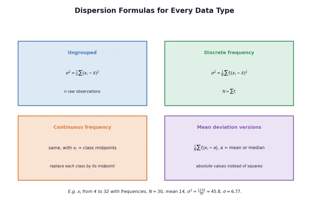
When values repeat, weight every deviation by its frequency:

Key Point (Discrete frequency distribution): with $N = \sum f_i$,

$$\bar{x} = \frac{1}{N}\sum f_ix_i, \qquad \sigma = \sqrt{\frac{1}{N}\sum f_i(x_i - \bar{x})^2}$$

Worked check: $x_i = 4, 8, 11, 17, 20, 24, 32$ with $f_i = 3, 5, 9, 5, 4, 3, 1$: $N = 30$, $\sum f_ix_i = 420$ so $\bar{x} = 14$; $\sum f_i(x_i - \bar{x})^2 = 1374$ so $\sigma^2 = 45.8$ and $\sigma \approx 6.77$.

Continuous frequency distributions: replace each class by its midpoint and proceed exactly as in the discrete case. (Gapped classes get the half-unit continuity correction first.)

There is also a frequency version of the computing identity:

$$\sigma^2 = \frac{1}{N}\sum f_ix_i^2 - \left(\frac{1}{N}\sum f_ix_i\right)^2 = \frac{1}{N^2}\left[N\sum f_ix_i^2 - \left(\sum f_ix_i\right)^2\right]$$

useful when the $x_i$ are small; when they are large, the shortcut method below is faster still.

The Shortcut (Step-Deviation) Method

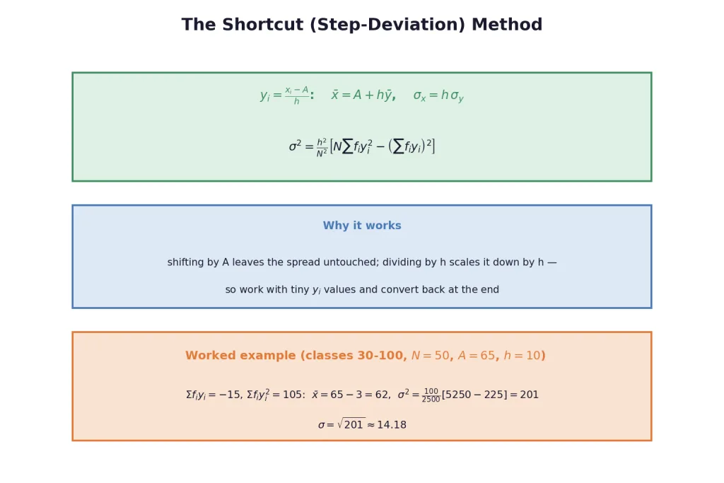
Large midpoints make direct computation tedious. Shift by an assumed mean $A$ (usually a middle midpoint) and shrink by the class width $h$:

Key Point (Step deviations): with $y_i = \frac{x_i - A}{h}$,

$$\bar{x} = A + h\bar{y} \qquad \sigma_x = h\,\sigma_y \qquad \sigma^2 = \frac{h^2}{N^2}\left[N\sum f_iy_i^2 - \left(\sum f_iy_i\right)^2\right]$$

Why it works: shifting every observation by $A$ moves the mean but leaves the spread untouched; dividing by $h$ scales the spread down by exactly $h$. So the tiny $y_i$ (typically $-3, -2, -1, 0, 1, 2, 3$) carry all the information, and one multiplication at the end converts back.

Worked example (classes 30-40 to 90-100 with frequencies 3, 7, 12, 15, 8, 3, 2; $A = 65$, $h = 10$): the table gives $\sum f_iy_i = -15$ and $\sum f_iy_i^2 = 105$, so

$$\bar{x} = 65 - \frac{15}{50} \times 10 = 62, \qquad \sigma^2 = \frac{100}{2500}\left[50(105) - (-15)^2\right] = 201, \qquad \sigma \approx 14.18$$

[Board Tip] Choose $A$ as the midpoint of a central class so the $y_i$ straddle zero — the sums stay small and sign errors stay visible. And remember the final multiply by $h$ for $\sigma$ (or $h^2$ for $\sigma^2$): forgetting it is the single most common shortcut-method error.

Solved Examples

Example 1: Discrete frequency distribution

Find the variance and SD for $x_i$: 4, 8, 11, 17, 20, 24, 32 with $f_i$: 3, 5, 9, 5, 4, 3, 1.

Solution:

Step 1 — Weighted mean. $N = 30$, $\sum f_ix_i = 420$: $\bar{x} = 14$.

Step 2 — Weighted squared deviations. $\sum f_i(x_i - 14)^2 = 1374$.

Step 3 — Divide and root. $\sigma^2 = \frac{1374}{30} = 45.8$; $\sigma \approx 6.77$.

Takeaway: The frequency column multiplies EVERY squared deviation — a five-column table ($x_i$, $f_i$, $f_ix_i$, $x_i - \bar{x}$, $f_i(x_i-\bar{x})^2$) keeps it honest.

Example 2: Mean and variance, discrete data

$x_i$: 6, 10, 14, 18, 24, 28, 30 with $f_i$: 2, 4, 7, 12, 8, 4, 3.

Solution:

Step 1 — Mean. $N = 40$, $\sum f_ix_i = 760$: $\bar{x} = 19$.

Step 2 — Weighted squares. $\sum f_i(x_i - 19)^2 = 1736$.

Step 3 — Divide. $\sigma^2 = \frac{1736}{40} = 43.4$.

Takeaway: A round mean (19 here) is the designer's gift — deviations stay integer and the table stays clean.

Example 3: Decimals welcome

$x_i$: 92, 93, 97, 98, 102, 104, 109 with $f_i$: 3, 2, 3, 2, 6, 3, 3.

Solution:

Step 1 — Mean. $N = 22$, $\sum f_ix_i = 2200$: $\bar{x} = 100$.

Step 2 — Weighted squares. $\sum f_i(x_i - 100)^2 = 3(64) + 2(49) + 3(9) + 2(4) + 6(4) + 3(16) + 3(81) = 640$.

Step 3 — Divide. $\sigma^2 = \frac{640}{22} \approx 29.09$.

Takeaway: Large $x_i$ values with a round mean still compute quickly — deviations, not raw values, do the work.

Example 4: Shortcut with $h = 1$

$x_i$: 60 to 68 with $f_i$: 2, 1, 12, 29, 25, 12, 10, 4, 5. Find the mean and SD by the shortcut method.

Solution:

Step 1 — Shift by $A = 64$. Deviations $d_i = x_i - 64$ run $-4$ to $4$; $N = 100$.

Step 2 — The lucky sum. $\sum f_id_i = 0$: $\bar{x} = 64 + 0 = 64$ exactly.

Step 3 — Spread. $\sum f_id_i^2 = 286$: $\sigma^2 = \frac{286}{100} - 0 = 2.86$, $\sigma \approx 1.69$.

Takeaway: With $h = 1$ the shortcut is a pure shift — and when $\sum f_id_i = 0$, the assumed mean IS the mean.

Example 5: Wide classes

Classes 0-30 up to 180-210 with frequencies 2, 3, 5, 10, 3, 5, 2. Find the mean and variance.

Solution:

Step 1 — Set up steps. Midpoints 15, 45, up to 195; $A = 105$, $h = 30$, $N = 30$.

Step 2 — Small sums. $\sum f_iy_i = 2$, $\sum f_iy_i^2 = 76$: $\bar{x} = 105 + \frac{2}{30} \times 30 = 107$.

Step 3 — Variance. $\sigma^2 = \frac{30^2}{30^2}\left[30(76) - 2^2\right] = 2280 - 4 = 2276$.

Takeaway: With $h = 30$ the raw numbers would be enormous — the shortcut trades them for single digits and one rescale.

Example 6: A compact continuous table

Classes 0-10 up to 40-50 with frequencies 5, 8, 15, 16, 6. Find the mean and variance.

Solution:

Step 1 — Midpoints. $5, 15, 25, 35, 45$; $N = 50$.

Step 2 — Mean. $\sum f_ix_i = 1350$: $\bar{x} = 27$.

Step 3 — Weighted squares. $\sum f_i(x_i - 27)^2 = 5(484) + 8(144) + 15(4) + 16(64) + 6(324) = 6600$: $\sigma^2 = 132$.

Takeaway: Direct computation stays feasible when midpoints are small — the shortcut is a choice, not a ritual.

Example 7: The full shortcut

Classes 30-40 up to 90-100 with frequencies 3, 7, 12, 15, 8, 3, 2. Find the mean, variance and SD.

Solution:

Step 1 — Steps about the middle. $A = 65$, $h = 10$, $N = 50$: the $y_i$ run $-3$ to $3$.

Step 2 — Sums. $\sum f_iy_i = -15$, $\sum f_iy_i^2 = 105$: $\bar{x} = 65 + \frac{-15}{50} \times 10 = 62$.

Step 3 — Variance and SD. $\sigma^2 = \frac{10^2}{50^2}\left[50(105) - (-15)^2\right] = \frac{100}{2500}(5250 - 225) = 201$: $\sigma = \sqrt{201} \approx 14.18$.

Takeaway: Note $(-15)^2 = +225$ is SUBTRACTED — squaring the negative sum then subtracting it is where sign discipline pays.

Example 8: Heights by shortcut

Heights (cm): classes 70-75 up to 110-115 with frequencies 3, 4, 7, 7, 15, 9, 6, 6, 3.

Solution:

Step 1 — Steps. Midpoints 72.5 up to 112.5; $A = 92.5$, $h = 5$, $N = 60$.

Step 2 — Mean. $\sum f_iy_i = 6$: $\bar{x} = 92.5 + \frac{6}{60} \times 5 = 93$ cm.

Step 3 — Variance. $\sum f_iy_i^2 = 254$: $\sigma^2 = \frac{25}{3600}\left[60(254) - 36\right] = \frac{25 \times 15204}{3600} \approx 105.58$: $\sigma \approx 10.27$ cm.

Takeaway: Half-unit midpoints (72.5, 77.5) vanish into clean integers under the step substitution — exactly what it is for.

Example 9: Continuity correction first

Diameters (mm): 33-36, 37-40, 41-44, 45-48, 49-52 with frequencies 15, 17, 21, 22, 25.

Solution:

Step 1 — Close the gaps. Classes become 32.5-36.5 and so on; midpoints $34.5, 38.5, 42.5, 46.5, 50.5$; $N = 100$.

Step 2 — Steps. $A = 42.5$, $h = 4$: $\sum f_iy_i = 25$, $\sum f_iy_i^2 = 199$; $\bar{x} = 42.5 + \frac{25}{100} \times 4 = 43.5$ mm.

Step 3 — Variance. $\sigma^2 = \frac{16}{10000}\left[100(199) - 625\right] = \frac{16 \times 19275}{10000} \approx 30.84$: $\sigma \approx 5.55$ mm.

Takeaway: Gapped classes get the half-unit correction BEFORE anything else — midpoints shift with it, and so does every downstream number.

Example 10: Reading the shortcut backwards

A distribution has $h = 10$, $N = 40$, $\sum f_iy_i = 8$, $\sum f_iy_i^2 = 50$ about $A = 55$. Find the mean and variance.

Solution:

Step 1 — Mean. $\bar{x} = 55 + \frac{8}{40} \times 10 = 57$.

Step 2 — Variance. $\sigma^2 = \frac{100}{1600}\left[40(50) - 8^2\right] = \frac{100 \times 1936}{1600} = 121$.

Step 3 — SD. $\sigma = 11$.

Takeaway: The four summary numbers $(A, h, \sum f_iy_i, \sum f_iy_i^2)$ carry the whole distribution's mean and spread — JEE often hands you exactly these.