Solved Examples

Solved Examples — the Full Chapter Workout

Thirty worked problems: scaling and shifting laws, missing observations, corrected statistics, then drills across every formula. Attempt each before reading the solution.

Example 1: Scaling observations

The variance of 20 observations is 5. Each observation is multiplied by 2. Find the new variance.

Solution:

Step 1 — Track the deviations. With $y_i = 2x_i$, the mean doubles too, so $y_i - \bar{y} = 2(x_i - \bar{x})$: every deviation doubles.

Step 2 — Square. Every squared deviation quadruples.

Step 3 — Conclude. New variance $= 2^2 \times 5 = 20$.

Takeaway: Multiplying data by $k$ multiplies the variance by $k^2$ (and the SD by $|k|$) — the scaling law in one line.

Example 2: Two missing observations

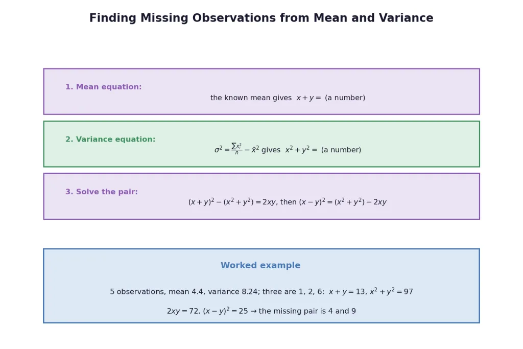
Five observations have mean 4.4 and variance 8.24; three of them are 1, 2, 6. Find the other two.

Solution:

Step 1 — Mean equation. $\sum x_i = 5 \times 4.4 = 22$; the knowns give 9: $x + y = 13$.

Step 2 — Variance equation. $\sum x_i^2 = n(\sigma^2 + \bar{x}^2) = 5(8.24 + 19.36) = 138$; the knowns give $1 + 4 + 36 = 41$: $x^2 + y^2 = 97$.

Step 3 — Solve the pair. $2xy = 13^2 - 97 = 72$; $(x - y)^2 = 97 - 72 = 25$, so $x - y = \pm 5$: the observations are 4 and 9.

Takeaway: Mean gives $x + y$, variance gives $x^2 + y^2$, and the identity $(x-y)^2 = (x^2 + y^2) - 2xy$ finishes — the standard three-step template.

Example 3: Shifting observations

Show that adding a constant $a$ to every observation leaves the variance unchanged.

Solution:

Step 1 — Shift the mean. $y_i = x_i + a$ gives $\bar{y} = \bar{x} + a$.

Step 2 — Compare deviations. $y_i - \bar{y} = (x_i + a) - (\bar{x} + a) = x_i - \bar{x}$ — identical.

Step 3 — Conclude. Identical deviations, identical variance. ∎

Takeaway: Variance is blind to location — only the spread pattern matters, which is why the shortcut method's shift by $A$ is free.

Example 4: Correcting a wrong entry

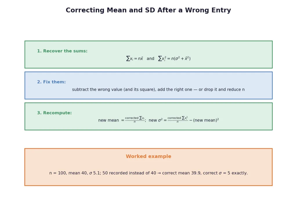
For 100 observations a student computed mean 40 and SD 5.1, having entered 50 instead of 40 once. Find the correct mean and SD.

Solution:

Step 1 — Recover the sums. $\sum x_i = 100 \times 40 = 4000$; $\sum x_i^2 = 100(5.1^2 + 40^2) = 100(26.01 + 1600) = 162601$.

Step 2 — Fix them. $\sum x_i \to 4000 - 50 + 40 = 3990$: correct mean 39.9. $\sum x_i^2 \to 162601 - 2500 + 1600 = 161701$.

Step 3 — Recompute. $\sigma^2 = \frac{161701}{100} - 39.9^2 = 1617.01 - 1592.01 = 25$: correct $\sigma = 5$ exactly.

Takeaway: Wrong-entry problems live entirely in the two sums — fix $\sum x_i$ and $\sum x_i^2$, then rebuild mean and SD from scratch.

Example 5: Missing pair, variant one

Eight observations have mean 9 and variance 9.25; six are 6, 7, 10, 12, 12, 13. Find the other two.

Solution:

Step 1 — Mean equation. $\sum x_i = 72$; knowns give 60: $x + y = 12$.

Step 2 — Variance equation. $\sum x_i^2 = 8(9.25 + 81) = 722$; knowns give $36+49+100+144+144+169 = 642$: $x^2 + y^2 = 80$.

Step 3 — Solve. $2xy = 144 - 80 = 64$; $(x-y)^2 = 80 - 64 = 16$: the observations are 4 and 8.

Takeaway: The template never changes — only the arithmetic; always check the pair satisfies BOTH original equations.

Example 6: Missing pair, variant two

Seven observations have mean 8 and variance 16; five are 2, 4, 10, 12, 14. Find the other two.

Solution:

Step 1 — Mean equation. $\sum x_i = 56$; knowns give 42: $x + y = 14$.

Step 2 — Variance equation. $\sum x_i^2 = 7(16 + 64) = 560$; knowns give $4+16+100+144+196 = 460$: $x^2 + y^2 = 100$.

Step 3 — Solve. $2xy = 196 - 100 = 96$; $(x-y)^2 = 4$: the observations are 6 and 8.

Takeaway: $(x+y)^2 - (x^2+y^2) = 2xy$ then $(x^2+y^2) - 2xy = (x-y)^2$ — two subtractions crack every missing-pair problem.

Example 7: Scale by 3

Six observations have mean 8 and SD 4. Each is multiplied by 3. Find the new mean and SD.

Solution:

Step 1 — Mean scales. $3 \times 8 = 24$.

Step 2 — SD scales by the absolute factor. $|3| \times 4 = 12$.

Takeaway: Mean and SD both scale linearly; only the VARIANCE picks up the square ($9 \times 16 = 144$ here).

Example 8: The general scaling law

Prove that $ax_1, \ldots, ax_n$ have mean $a\bar{x}$ and variance $a^2\sigma^2$.

Solution:

Step 1 — Mean. $\bar{y} = \frac{1}{n}\sum ax_i = a \cdot \frac{1}{n}\sum x_i = a\bar{x}$.

Step 2 — Deviations. $y_i - \bar{y} = a(x_i - \bar{x})$.

Step 3 — Variance. $\sigma_y^2 = \frac{1}{n}\sum a^2(x_i - \bar{x})^2 = a^2\sigma^2$. ∎

Takeaway: The factor $a$ comes OUT of the deviation before squaring — that is the whole proof, three lines.

Example 9: Wrong observation omitted

Twenty observations have mean 10 and SD 2. The observation 8 was wrong. Find the mean and SD if it is omitted.

Solution:

Step 1 — Fix the sums, reduce $n$. $\sum x_i = 200 - 8 = 192$ over $n = 19$: mean $= \frac{192}{19} \approx 10.11$.

Step 2 — Fix the squares. $\sum x_i^2 = 20(4 + 100) = 2080 \to 2080 - 64 = 2016$.

Step 3 — Recompute. $\sigma^2 = \frac{2016}{19} - \left(\frac{192}{19}\right)^2 \approx 106.11 - 102.12 = 3.99$: $\sigma \approx 2.0$.

Takeaway: OMITTING an entry changes $n$ as well as the sums — the divisor drops to 19; replacement problems keep $n$ fixed.

Example 10: Wrong observation replaced

Same data, but 8 is replaced by 12.

Solution:

Step 1 — Fix the sum. $\sum x_i = 200 - 8 + 12 = 204$: mean $= \frac{204}{20} = 10.2$.

Step 2 — Fix the squares. $\sum x_i^2 = 2080 - 64 + 144 = 2160$.

Step 3 — Recompute. $\sigma^2 = \frac{2160}{20} - 10.2^2 = 108 - 104.04 = 3.96$: $\sigma \approx 1.99$.

Takeaway: Replace = subtract the wrong value (and its square), add the right one, SAME $n$ — contrast with Example 9's omission.

Example 11: Three wrong entries omitted

100 observations have mean 20 and SD 3. Three entries 21, 21, 18 were incorrect. Find the mean and SD with them omitted.

Solution:

Step 1 — Fix the sum. $\sum x_i = 2000 - (21 + 21 + 18) = 1940$ over $n = 97$: mean $= \frac{1940}{97} = 20$ exactly.

Step 2 — Fix the squares. $\sum x_i^2 = 100(9 + 400) = 40900 \to 40900 - (441 + 441 + 324) = 39694$.

Step 3 — Recompute. $\sigma^2 = \frac{39694}{97} - 400 \approx 409.22 - 400 = 9.22$: $\sigma \approx 3.04$.

Takeaway: The omitted values averaged exactly 20, so the mean survived untouched — but the SD still moved; check both, never assume.

Example 12: SD versus M.D. on the same data

For $4, 7, 8, 9, 10, 12, 13, 17$ (mean 10, M.D. 3), find $\sigma$ and compare.

Solution:

Step 1 — Sum of squares. $\sum x_i^2 = 16+49+64+81+100+144+169+289 = 912$.

Step 2 — Identity. $\sigma^2 = \frac{912}{8} - 100 = 114 - 100 = 14$: $\sigma = \sqrt{14} \approx 3.74$.

Step 3 — Compare. $\sigma \approx 3.74 > 3 =$ M.D.

Takeaway: Squaring weights large deviations more heavily than absolute values do — $\sigma \geq$ M.D. is the typical picture.

Example 13: Even numbers

Find the mean and variance of the first 10 even natural numbers $2, 4, \ldots, 20$.

Solution:

Step 1 — Scaling view. The data is $2 \times (1, 2, \ldots, 10)$.

Step 2 — Mean. $2 \times \frac{11}{2} = 11$.

Step 3 — Variance. $2^2 \times \frac{10^2 - 1}{12} = 4 \times 8.25 = 33$.

Takeaway: Even naturals = doubled naturals — quote the standard result and scale, no tables needed.

Example 14: A constant data set

Find the SD of $5, 5, 5, 5, 5$.

Solution:

Step 1 — Mean. Obviously 5.

Step 2 — Deviations. All zero.

Step 3 — Conclude. $\sigma = 0$ — the only way SD vanishes.

Takeaway: Zero SD characterises constant data; any variety at all forces $\sigma > 0$.

Example 15: Recovering $\sum x_i^2$

Twenty observations have mean 10 and SD 3. Find $\sum x_i^2$.

Solution:

Step 1 — Rearrange the identity. $\sigma^2 = \frac{\sum x_i^2}{n} - \bar{x}^2$ gives $\sum x_i^2 = n(\sigma^2 + \bar{x}^2)$.

Step 2 — Substitute. $= 20(9 + 100) = 2180$.

Takeaway: $(n, \bar{x}, \sigma)$ and $(n, \sum x_i, \sum x_i^2)$ are interchangeable data — convert freely in either direction.

Example 16: Mean of squares

A data set has mean 6 and variance 4. Find the mean of the squares of the observations.

Solution:

Step 1 — Rearrange. $\overline{x^2} = \sigma^2 + \bar{x}^2$.

Step 2 — Substitute. $= 4 + 36 = 40$.

Takeaway: Mean of squares $\ne$ square of mean — they differ by exactly the variance; that gap IS the definition.

Example 17: A symmetric set

Find the variance of $-3, -2, -1, 0, 1, 2, 3$.

Solution:

Step 1 — Shift view. This is $1, 2, \ldots, 7$ shifted by $-4$.

Step 2 — Shifts preserve variance. $\sigma^2 = \frac{7^2 - 1}{12} = 4$.

Step 3 — Direct check. $\frac{9+4+1+0+1+4+9}{7} = \frac{28}{7} = 4$ ✓ (mean 0 makes the check one line).

Takeaway: Recognising a data set as a shift of a standard one converts computation into recall.

Example 18: Shift by 5

Data has mean 12 and variance 7. Every observation is increased by 5. New mean and variance?

Solution:

Step 1 — Mean shifts. $12 + 5 = 17$.

Step 2 — Variance ignores shifts. Still 7.

Takeaway: Location moves, spread stays — the shift law's whole content.

Example 19: Scale by $-2$

Data has mean 12 and SD 3. Every observation is multiplied by $-2$. New mean and SD?

Solution:

Step 1 — Mean scales with sign. $-2 \times 12 = -24$.

Step 2 — SD scales by the ABSOLUTE value. $|-2| \times 3 = 6$.

Step 3 — Sanity. SD is never negative, whatever the multiplier's sign.

Takeaway: $\sigma_y = |a|\sigma_x$ — the modulus in the scaling law exists precisely for negative multipliers.

Example 20: M.D. about the median, fresh data

Find the M.D. about the median of $3, 9, 5, 3, 12, 10, 18, 4, 7, 19, 21$.

Solution:

Step 1 — Sort and pick the middle. Sorted: $3, 3, 4, 5, 7, 9, 10, 12, 18, 19, 21$; with $n = 11$ the median is the 6th value: 9.

Step 2 — Absolute deviations. $6+6+5+4+2+0+1+3+9+10+12 = 58$.

Step 3 — Average. M.D. $= \frac{58}{11} \approx 5.27$.

Takeaway: Odd $n$ gives a single middle observation — no averaging of two central values needed.

Example 21: First $n$ even naturals in general

Show that the variance of $2, 4, \ldots, 2n$ is $\frac{n^2 - 1}{3}$.

Solution:

Step 1 — Scaling view. The data is $2 \times (1, \ldots, n)$.

Step 2 — Scale the standard result. $\sigma^2 = 4 \times \frac{n^2 - 1}{12}$.

Step 3 — Simplify. $= \frac{n^2 - 1}{3}$. ∎

Takeaway: New "standard results" are old ones passed through the scaling law — derive, don't memorise separately.

Example 22: Identity drill

Ten observations satisfy $\sum x_i = 50$ and $\sum x_i^2 = 290$. Find $\sigma$.

Solution:

Step 1 — Mean. $\bar{x} = 5$.

Step 2 — Identity. $\sigma^2 = \frac{290}{10} - 25 = 4$.

Step 3 — Root. $\sigma = 2$.

Takeaway: Two sums in, SD out — the computing identity is a two-line machine.

Example 23: Scale then shift

The variance of 10 observations is 5. Each is doubled and then 3 is added. Find the new variance.

Solution:

Step 1 — The shift contributes nothing. $+3$ is invisible to variance.

Step 2 — The scale contributes its square. $2^2 = 4$.

Step 3 — Conclude. New variance $= 4 \times 5 = 20$.

Takeaway: For $y = ax + b$: $\sigma_y^2 = a^2\sigma_x^2$ — the $b$ NEVER matters, whatever order the operations happen.

Example 24: A missing pair with round numbers

Five observations have mean 6 and variance 8; three of them are 2, 6, 10. Find the other two.

Solution:

Step 1 — Mean equation. $\sum x_i = 30$; knowns give 18: $x + y = 12$.

Step 2 — Variance equation. $\sum x_i^2 = 5(8 + 36) = 220$; knowns give $4 + 36 + 100 = 140$: $x^2 + y^2 = 80$.

Step 3 — Solve. $2xy = 144 - 80 = 64$; $(x-y)^2 = 16$: the pair is 4 and 8.

Takeaway: The same template as before, now with round numbers — speed comes from the ritual, not the values.

Example 25: A replacement correction

Twenty observations have mean 10 and SD 1. The value 8 was recorded instead of the correct 12. Find the corrected mean and SD.

Solution:

Step 1 — Fix the sum. $\sum x_i = 200 - 8 + 12 = 204$: mean $= 10.2$.

Step 2 — Fix the squares. $\sum x_i^2 = 20(1 + 100) = 2020 \to 2020 - 64 + 144 = 2100$.

Step 3 — Recompute. $\sigma^2 = \frac{2100}{20} - 10.2^2 = 105 - 104.04 = 0.96$: $\sigma \approx 0.98$.

Takeaway: A small SD magnifies the impact of one wrong entry — recompute honestly rather than assuming the correction is negligible.

Example 26: Two-value data

Find the SD of just two observations $a$ and $b$.

Solution:

Step 1 — Mean. $\frac{a+b}{2}$ — the midpoint.

Step 2 — Deviations. Each value sits $\frac{|a-b|}{2}$ from the midpoint (one above, one below).

Step 3 — SD. $\sigma = \sqrt{\frac{2 \cdot (a-b)^2/4}{2}} = \frac{|a - b|}{2}$ — half the gap.

Takeaway: For two points, SD = half the distance between them — a formula worth carrying into JEE.

Example 27: Range vs SD

For $48, 49, 50, 51, 52$: find the range and SD, and note the contrast.

Solution:

Step 1 — Range. $52 - 48 = 4$.

Step 2 — SD. $\sigma^2 = \frac{4+1+0+1+4}{5} = 2$: $\sigma = \sqrt{2} \approx 1.41$.

Step 3 — Contrast. The range sees only the two extremes; the SD weighs every observation.

Takeaway: Different measures answer different questions — the range is a quick bound, the SD a full census.

Example 28: Shift-invariance by the identity

Prove the shift law using $\sigma^2 = \overline{x^2} - \bar{x}^2$.

Solution:

Step 1 — Shifted mean of squares. For $y = x + a$: $\overline{y^2} = \overline{x^2} + 2a\bar{x} + a^2$.

Step 2 — Shifted squared mean. $\bar{y}^2 = (\bar{x} + a)^2 = \bar{x}^2 + 2a\bar{x} + a^2$.

Step 3 — Subtract. The cross terms cancel identically: $\sigma_y^2 = \overline{x^2} - \bar{x}^2 = \sigma_x^2$. ∎

Takeaway: The same law, proved two ways (deviations in Example 3, identity here) — cross-proofs are the cheapest error insurance.

Example 29: Frequency identity drill

A discrete distribution has $N = 25$, $\sum f_ix_i = 125$ and $\sum f_ix_i^2 = 725$. Find $\sigma$.

Solution:

Step 1 — Mean. $\bar{x} = \frac{125}{25} = 5$.

Step 2 — Identity. $\sigma^2 = \frac{725}{25} - 25 = 29 - 25 = 4$.

Step 3 — Root. $\sigma = 2$.

Takeaway: The frequency version of the identity works the same — $f_i$-weighted sums replace plain sums, $N$ replaces $n$.

Example 30: A capstone check

The mean of $1, 3, 5, 7, 9$ is 5. Verify that its variance equals that of $11, 13, 15, 17, 19$.

Solution:

Step 1 — Spot the shift. The second set is the first plus 10 — variance must match.

Step 2 — Compute once. Odd numbers $2k - 1$ ($k = 1, \ldots, 5$) are scaled-shifted naturals: $\sigma^2 = 2^2 \times \frac{5^2 - 1}{12} = 8$.

Step 3 — Confirm directly. Deviations from 5: $\pm 4, \pm 2, 0$ — squares sum to 40, $\frac{40}{5} = 8$ ✓ for both sets.

Takeaway: Scaling and shift laws let one computation certify two data sets — the chapter's toolkit working as a system.