The Limit Laws
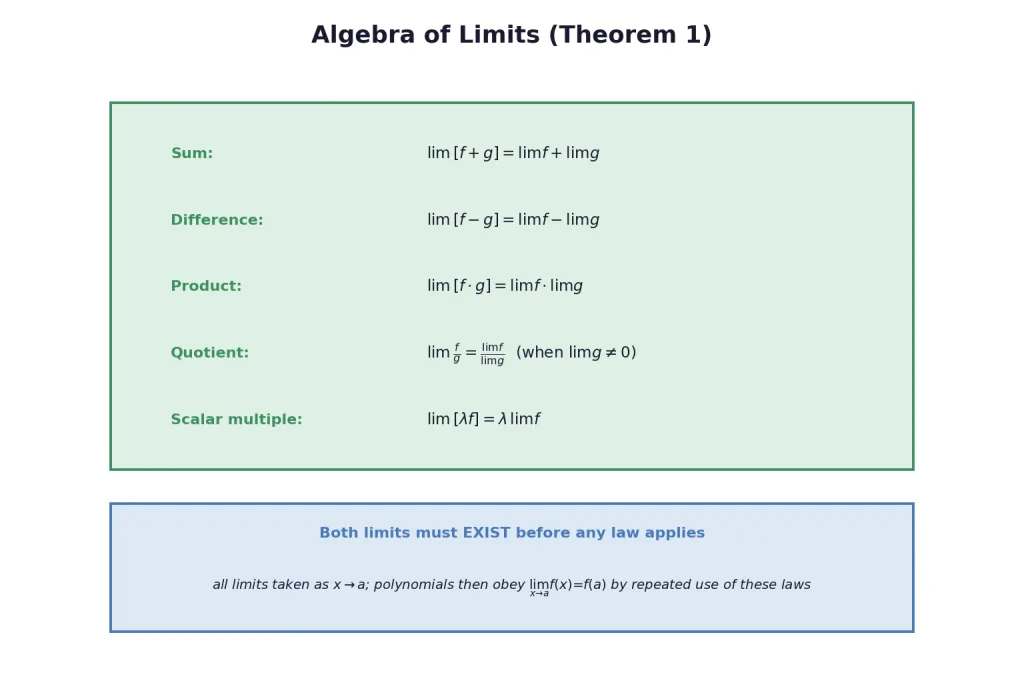
Limits respect arithmetic. If lim x → a f ( x ) \lim_{x \to a} f(x) lim x → a f ( x ) lim x → a g ( x ) \lim_{x \to a} g(x) lim x → a g ( x )
Key Point (Theorem 1): lim [ f ± g ] = lim f ± lim g \lim [f \pm g] = \lim f \pm \lim g lim [ f ± g ] = lim f ± lim g lim [ f ⋅ g ] = lim f ⋅ lim g \lim [f \cdot g] = \lim f \cdot \lim g lim [ f ⋅ g ] = lim f ⋅ lim g lim f g = lim f lim g \lim \frac{f}{g} = \frac{\lim f}{\lim g} lim g f = l i m g l i m f lim g ≠ 0 \lim g \ne 0 lim g = 0 lim [ λ f ] = λ lim f \lim [\lambda f] = \lambda \lim f lim [ λ f ] = λ lim f λ \lambda λ
Polynomials: just substitute. Since lim x → a x = a \lim_{x \to a} x = a lim x → a x = a lim x → a x n = a n \lim_{x \to a} x^n = a^n lim x → a x n = a n
lim x → a f ( x ) = f ( a ) for every polynomial f \lim_{x \to a} f(x) = f(a) \quad \text{for every polynomial } f x → a lim f ( x ) = f ( a ) for every polynomial f
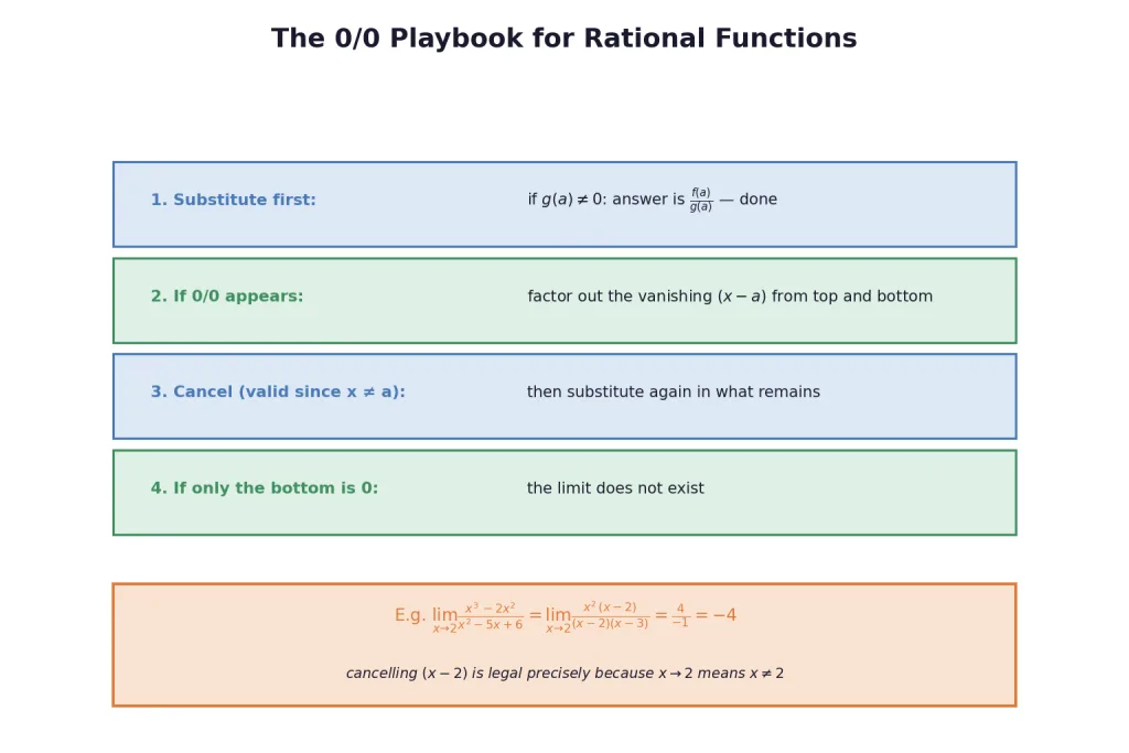
Rational functions g ( x ) h ( x ) \frac{g(x)}{h(x)} h ( x ) g ( x ) h ( a ) ≠ 0 h(a) \ne 0 h ( a ) = 0 g ( a ) h ( a ) \frac{g(a)}{h(a)} h ( a ) g ( a ) h ( a ) = 0 h(a) = 0 h ( a ) = 0 g ( a ) ≠ 0 g(a) \ne 0 g ( a ) = 0 both vanish — the 0 0 \frac{0}{0} 0 0 ( x − a ) (x - a) ( x − a )
Cancelling ( x − a ) (x - a) ( x − a ) x → a x \to a x → a x ≠ a x \ne a x = a
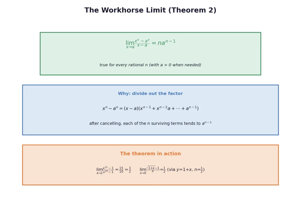
The Workhorse: lim x → a x n − a n x − a = n a n − 1 \lim_{x \to a} \frac{x^n - a^n}{x - a} = na^{n-1} lim x → a x − a x n − a n = n a n − 1
Key Point (Theorem 2): for any positive integer n n n n n n a > 0 a > 0 a > 0
lim x → a x n − a n x − a = n a n − 1 \lim_{x \to a} \frac{x^n - a^n}{x - a} = na^{n-1} x → a lim x − a x n − a n = n a n − 1
Why: x n − a n = ( x − a ) ( x n − 1 + x n − 2 a + ⋯ + a n − 1 ) x^n - a^n = (x - a)(x^{n-1} + x^{n-2}a + \cdots + a^{n-1}) x n − a n = ( x − a ) ( x n − 1 + x n − 2 a + ⋯ + a n − 1 ) n n n a n − 1 a^{n-1} a n − 1
Using it: lim x → 1 x 15 − 1 x 10 − 1 \lim_{x \to 1} \frac{x^{15} - 1}{x^{10} - 1} lim x → 1 x 10 − 1 x 15 − 1 x − 1 x - 1 x − 1 15 10 = 3 2 \frac{15}{10} = \frac{3}{2} 10 15 = 2 3 lim x → 0 1 + x − 1 x \lim_{x \to 0} \frac{\sqrt{1 + x} - 1}{x} lim x → 0 x 1 + x − 1 y = 1 + x y = 1 + x y = 1 + x lim y → 1 y 1 / 2 − 1 y − 1 = 1 2 \lim_{y \to 1} \frac{y^{1/2} - 1}{y - 1} = \frac{1}{2} lim y → 1 y − 1 y 1/2 − 1 = 2 1
Recognition drill: any limit of the shape ( power ) − ( same power at a ) x − a \frac{(\text{power}) - (\text{same power at } a)}{x - a} x − a ( power ) − ( same power at a ) ( x + 1 ) 5 − 1 x \frac{(x+1)^5 - 1}{x} x ( x + 1 ) 5 − 1 y = x + 1 y = x + 1 y = x + 1
[Board Tip] Quote the theorem by name-and-statement when you use it — "by lim x → a x n − a n x − a = n a n − 1 \lim_{x \to a}\frac{x^n - a^n}{x - a} = na^{n-1} lim x → a x − a x n − a n = n a n − 1
Solved Examples
Example 1: Polynomials by substitution
Find: (i) lim x → 1 [ x 3 − x 2 + 1 ] \lim_{x \to 1}[x^3 - x^2 + 1] lim x → 1 [ x 3 − x 2 + 1 ] lim x → 3 [ x ( x + 1 ) ] \lim_{x \to 3}[x(x + 1)] lim x → 3 [ x ( x + 1 )] lim x → − 1 [ 1 + x + x 2 + ⋯ + x 10 ] \lim_{x \to -1}[1 + x + x^2 + \cdots + x^{10}] lim x → − 1 [ 1 + x + x 2 + ⋯ + x 10 ]
Solution:
Step 1 — (i) Substitute. Polynomials obey lim = \lim = lim = 1 − 1 + 1 = 1 1 - 1 + 1 = 1 1 − 1 + 1 = 1
Step 2 — (ii). 3 × ( 3 + 1 ) = 12 3 \times (3 + 1) = 12 3 × ( 3 + 1 ) = 12
Step 3 — (iii) Count the alternation. At x = − 1 x = -1 x = − 1 1 − 1 + 1 − ⋯ + 1 1 - 1 + 1 - \cdots + 1 1 − 1 + 1 − ⋯ + 1 + 1 +1 + 1
Takeaway: For any polynomial, the limit is one substitution; the only care needed is arithmetic, as in the alternating sum.
Example 2: Direct substitution
Evaluate: (i) lim x → 3 ( x + 3 ) \lim_{x \to 3}(x + 3) lim x → 3 ( x + 3 ) lim x → π ( x − 22 7 ) \lim_{x \to \pi}\left(x - \frac{22}{7}\right) lim x → π ( x − 7 22 ) lim r → 1 π r 2 \lim_{r \to 1} \pi r^2 lim r → 1 π r 2
Solution:
Step 1 — (i). 3 + 3 = 6 3 + 3 = 6 3 + 3 = 6
Step 2 — (ii). π − 22 7 \pi - \frac{22}{7} π − 7 22 22 7 = 3.142857 … \frac{22}{7} = 3.142857\ldots 7 22 = 3.142857 … π = 3.14159 … \pi = 3.14159\ldots π = 3.14159 …
Step 3 — (iii). π ( 1 ) 2 = π \pi(1)^2 = \pi π ( 1 ) 2 = π
Takeaway: Part (ii) is a designed trap — π ≠ 22 7 \pi \ne \frac{22}{7} π = 7 22
Example 3: Rational, denominator alive
Evaluate: (i) lim x → 4 4 x + 3 x − 2 \lim_{x \to 4} \frac{4x + 3}{x - 2} lim x → 4 x − 2 4 x + 3 lim x → − 1 x 10 + x 5 + 1 x − 1 \lim_{x \to -1} \frac{x^{10} + x^5 + 1}{x - 1} lim x → − 1 x − 1 x 10 + x 5 + 1
Solution:
Step 1 — Check the denominator FIRST. (i) At 4: x − 2 = 2 ≠ 0 x - 2 = 2 \ne 0 x − 2 = 2 = 0
Step 2 — (i) Substitute. 16 + 3 2 = 19 2 \frac{16 + 3}{2} = \frac{19}{2} 2 16 + 3 = 2 19
Step 3 — (ii) Same check, then substitute. Denominator − 2 ≠ 0 -2 \ne 0 − 2 = 0 1 − 1 + 1 − 2 = − 1 2 \frac{1 - 1 + 1}{-2} = -\frac{1}{2} − 2 1 − 1 + 1 = − 2 1
Takeaway: A rational limit begins with one question — is the denominator non-zero at the point? If yes, it is a substitution problem.
Example 4: The 0/0 factor-cancel
Evaluate: (i) lim x → 2 x 3 − 4 x 2 + 4 x x 2 − 4 \lim_{x \to 2} \frac{x^3 - 4x^2 + 4x}{x^2 - 4} lim x → 2 x 2 − 4 x 3 − 4 x 2 + 4 x lim x → 2 x 2 − 4 x 3 − 4 x 2 + 4 x \lim_{x \to 2} \frac{x^2 - 4}{x^3 - 4x^2 + 4x} lim x → 2 x 3 − 4 x 2 + 4 x x 2 − 4 lim x → 2 x 3 − 2 x 2 x 2 − 5 x + 6 \lim_{x \to 2} \frac{x^3 - 2x^2}{x^2 - 5x + 6} lim x → 2 x 2 − 5 x + 6 x 3 − 2 x 2
Solution:
Step 1 — (i) Factor out the vanishing power. x ( x − 2 ) 2 ( x + 2 ) ( x − 2 ) = x ( x − 2 ) x + 2 \frac{x(x-2)^2}{(x+2)(x-2)} = \frac{x(x-2)}{x+2} ( x + 2 ) ( x − 2 ) x ( x − 2 ) 2 = x + 2 x ( x − 2 ) 2 × 0 4 = 0 \frac{2 \times 0}{4} = 0 4 2 × 0 = 0
Step 2 — (ii) The reciprocal flips the story. ( x + 2 ) ( x − 2 ) x ( x − 2 ) 2 = x + 2 x ( x − 2 ) → 4 0 \frac{(x+2)(x-2)}{x(x-2)^2} = \frac{x+2}{x(x-2)} \to \frac{4}{0} x ( x − 2 ) 2 ( x + 2 ) ( x − 2 ) = x ( x − 2 ) x + 2 → 0 4
Step 3 — (iii) Factor and cancel once. x 2 ( x − 2 ) ( x − 2 ) ( x − 3 ) = x 2 x − 3 → 4 − 1 = − 4 \frac{x^2(x-2)}{(x-2)(x-3)} = \frac{x^2}{x-3} \to \frac{4}{-1} = -4 ( x − 2 ) ( x − 3 ) x 2 ( x − 2 ) = x − 3 x 2 → − 1 4 = − 4
Takeaway: After cancelling, re-substitute and READ the form: 0 4 \frac{0}{4} 4 0 4 0 \frac{4}{0} 0 4 4 − 1 \frac{4}{-1} − 1 4
Example 5: Combine first, then cancel
Evaluate lim x → 1 [ x − 2 x 2 − x − 1 x 3 − 3 x 2 + 2 x ] \lim_{x \to 1}\left[\frac{x - 2}{x^2 - x} - \frac{1}{x^3 - 3x^2 + 2x}\right] lim x → 1 [ x 2 − x x − 2 − x 3 − 3 x 2 + 2 x 1 ]
Solution:
Step 1 — Factor the denominators. x 2 − x = x ( x − 1 ) x^2 - x = x(x-1) x 2 − x = x ( x − 1 ) x 3 − 3 x 2 + 2 x = x ( x − 1 ) ( x − 2 ) x^3 - 3x^2 + 2x = x(x-1)(x-2) x 3 − 3 x 2 + 2 x = x ( x − 1 ) ( x − 2 )
Step 2 — Combine over the common denominator x ( x − 1 ) ( x − 2 ) x(x-1)(x-2) x ( x − 1 ) ( x − 2 ) Numerator: ( x − 2 ) 2 − 1 = x 2 − 4 x + 3 = ( x − 3 ) ( x − 1 ) (x-2)^2 - 1 = x^2 - 4x + 3 = (x-3)(x-1) ( x − 2 ) 2 − 1 = x 2 − 4 x + 3 = ( x − 3 ) ( x − 1 )
Step 3 — Cancel and substitute. ( x − 3 ) ( x − 1 ) x ( x − 1 ) ( x − 2 ) = x − 3 x ( x − 2 ) → − 2 1 × ( − 1 ) = 2 \frac{(x-3)(x-1)}{x(x-1)(x-2)} = \frac{x-3}{x(x-2)} \to \frac{-2}{1 \times (-1)} = 2 x ( x − 1 ) ( x − 2 ) ( x − 3 ) ( x − 1 ) = x ( x − 2 ) x − 3 → 1 × ( − 1 ) − 2 = 2
Takeaway: When each piece separately blows up, combine into ONE fraction first — the infinities cancel on paper before they can mislead.
Example 6: Shifted powers and quadratics
Evaluate: (i) lim x → 0 ( x + 1 ) 5 − 1 x \lim_{x \to 0} \frac{(x+1)^5 - 1}{x} lim x → 0 x ( x + 1 ) 5 − 1 lim x → 2 3 x 2 − x − 10 x 2 − 4 \lim_{x \to 2} \frac{3x^2 - x - 10}{x^2 - 4} lim x → 2 x 2 − 4 3 x 2 − x − 10
Solution:
Step 1 — (i) Shift into workhorse form. Put y = x + 1 y = x + 1 y = x + 1 y → 1 y \to 1 y → 1 lim y → 1 y 5 − 1 y − 1 \lim_{y \to 1} \frac{y^5 - 1}{y - 1} lim y → 1 y − 1 y 5 − 1
Step 2 — (i) Apply the theorem. 5 ( 1 ) 4 = 5 5(1)^4 = 5 5 ( 1 ) 4 = 5
Step 3 — (ii) Factor the 0/0. ( x − 2 ) ( 3 x + 5 ) ( x − 2 ) ( x + 2 ) = 3 x + 5 x + 2 → 11 4 \frac{(x-2)(3x+5)}{(x-2)(x+2)} = \frac{3x+5}{x+2} \to \frac{11}{4} ( x − 2 ) ( x + 2 ) ( x − 2 ) ( 3 x + 5 ) = x + 2 3 x + 5 → 4 11
Takeaway: ( x + 1 ) n − 1 (x + 1)^n - 1 ( x + 1 ) n − 1 x x x
Example 7: Higher-degree factoring
Evaluate lim x → 3 x 4 − 81 2 x 2 − 5 x − 3 \lim_{x \to 3} \frac{x^4 - 81}{2x^2 - 5x - 3} lim x → 3 2 x 2 − 5 x − 3 x 4 − 81
Solution:
Step 1 — Factor top and bottom. x 4 − 81 = ( x 2 − 9 ) ( x 2 + 9 ) = ( x − 3 ) ( x + 3 ) ( x 2 + 9 ) x^4 - 81 = (x^2 - 9)(x^2 + 9) = (x-3)(x+3)(x^2+9) x 4 − 81 = ( x 2 − 9 ) ( x 2 + 9 ) = ( x − 3 ) ( x + 3 ) ( x 2 + 9 ) 2 x 2 − 5 x − 3 = ( x − 3 ) ( 2 x + 1 ) 2x^2 - 5x - 3 = (x-3)(2x+1) 2 x 2 − 5 x − 3 = ( x − 3 ) ( 2 x + 1 )
Step 2 — Cancel ( x − 3 ) (x - 3) ( x − 3 ) Left with ( x + 3 ) ( x 2 + 9 ) 2 x + 1 \frac{(x+3)(x^2+9)}{2x+1} 2 x + 1 ( x + 3 ) ( x 2 + 9 )
Step 3 — Substitute. 6 × 18 7 = 108 7 \frac{6 \times 18}{7} = \frac{108}{7} 7 6 × 18 = 7 108
Takeaway: Difference of squares twice (x 4 − 81 → x 2 − 9 → x − 3 x^4 - 81 \to x^2 - 9 \to x - 3 x 4 − 81 → x 2 − 9 → x − 3
Example 8: Parameters ride along
Evaluate: (i) lim x → 0 a x + b c x + 1 \lim_{x \to 0} \frac{ax + b}{cx + 1} lim x → 0 c x + 1 a x + b lim x → 1 a x 2 + b x + c c x 2 + b x + a \lim_{x \to 1} \frac{ax^2 + bx + c}{cx^2 + bx + a} lim x → 1 c x 2 + b x + a a x 2 + b x + c a + b + c ≠ 0 a + b + c \ne 0 a + b + c = 0
Solution:
Step 1 — (i) Denominator at 0. c ( 0 ) + 1 = 1 ≠ 0 c(0) + 1 = 1 \ne 0 c ( 0 ) + 1 = 1 = 0
Step 2 — (i) Read off. b 1 = b \frac{b}{1} = b 1 b = b
Step 3 — (ii) Substitute at 1. Top: a + b + c a + b + c a + b + c c + b + a c + b + a c + b + a a + b + c ≠ 0 a + b + c \ne 0 a + b + c = 0 0 0 \frac{0}{0} 0 0
Takeaway: Letters obey the same laws as numbers — check the denominator, substitute, simplify.
Example 9: Fractional powers via substitution
Evaluate lim z → 1 z 1 / 3 − 1 z 1 / 6 − 1 \lim_{z \to 1} \frac{z^{1/3} - 1}{z^{1/6} - 1} lim z → 1 z 1/6 − 1 z 1/3 − 1
Solution:
Step 1 — Clear the fractions with one substitution. Let z = t 6 z = t^6 z = t 6 z → 1 z \to 1 z → 1 t → 1 t \to 1 t → 1 z 1 / 3 = t 2 z^{1/3} = t^2 z 1/3 = t 2 z 1 / 6 = t z^{1/6} = t z 1/6 = t
Step 2 — Simplify. t 2 − 1 t − 1 = t + 1 \frac{t^2 - 1}{t - 1} = t + 1 t − 1 t 2 − 1 = t + 1 t ≠ 1 t \ne 1 t = 1
Step 3 — Conclude. The limit is 1 + 1 = 2 1 + 1 = 2 1 + 1 = 2 1 / 3 1 / 6 = 2 \frac{1/3}{1/6} = 2 1/6 1/3 = 2
Takeaway: For mixed fractional exponents substitute z = t k z = t^k z = t k k k k
Example 10: Combine, then cancel
Evaluate lim x → − 2 1 x + 1 2 x + 2 \lim_{x \to -2} \frac{\frac{1}{x} + \frac{1}{2}}{x + 2} lim x → − 2 x + 2 x 1 + 2 1
Solution:
Step 1 — Combine the numerator. 1 x + 1 2 = 2 + x 2 x \frac{1}{x} + \frac{1}{2} = \frac{2 + x}{2x} x 1 + 2 1 = 2 x 2 + x
Step 2 — Divide. x + 2 2 x ( x + 2 ) = 1 2 x \frac{x + 2}{2x(x + 2)} = \frac{1}{2x} 2 x ( x + 2 ) x + 2 = 2 x 1 x ≠ − 2 x \ne -2 x = − 2
Step 3 — Substitute. 1 2 ( − 2 ) = − 1 4 \frac{1}{2(-2)} = -\frac{1}{4} 2 ( − 2 ) 1 = − 4 1
Takeaway: The ( x + 2 ) (x + 2) ( x + 2 )
Example 11: The workhorse twice
Evaluate: (i) lim x → 1 x 15 − 1 x 10 − 1 \lim_{x \to 1} \frac{x^{15} - 1}{x^{10} - 1} lim x → 1 x 10 − 1 x 15 − 1 lim x → 0 1 + x − 1 x \lim_{x \to 0} \frac{\sqrt{1+x} - 1}{x} lim x → 0 x 1 + x − 1
Solution:
Step 1 — (i) Divide top and bottom by x − 1 x - 1 x − 1 ( x 15 − 1 ) / ( x − 1 ) ( x 10 − 1 ) / ( x − 1 ) → 15 ( 1 ) 14 10 ( 1 ) 9 \frac{(x^{15}-1)/(x-1)}{(x^{10}-1)/(x-1)} \to \frac{15(1)^{14}}{10(1)^9} ( x 10 − 1 ) / ( x − 1 ) ( x 15 − 1 ) / ( x − 1 ) → 10 ( 1 ) 9 15 ( 1 ) 14
Step 2 — (i) Simplify. 15 10 = 3 2 \frac{15}{10} = \frac{3}{2} 10 15 = 2 3
Step 3 — (ii) Shift to base 1. With y = 1 + x y = 1 + x y = 1 + x lim y → 1 y 1 / 2 − 1 y − 1 = 1 2 ( 1 ) − 1 / 2 = 1 2 \lim_{y \to 1} \frac{y^{1/2} - 1}{y - 1} = \frac{1}{2}(1)^{-1/2} = \frac{1}{2} lim y → 1 y − 1 y 1/2 − 1 = 2 1 ( 1 ) − 1/2 = 2 1
Takeaway: Splitting one ratio into two workhorse quotients (divide both by x − a x - a x − a x m − a m x n − a n \frac{x^m - a^m}{x^n - a^n} x n − a n x m − a m m n a m − n \frac{m}{n}a^{m-n} n m a m − n
Example 12: Workhorse with a general exponent
If lim x → 2 x n − 2 n x − 2 = 80 \lim_{x \to 2} \frac{x^n - 2^n}{x - 2} = 80 lim x → 2 x − 2 x n − 2 n = 80 n n n n n n
Solution:
Step 1 — Apply the theorem. The limit equals n ⋅ 2 n − 1 n \cdot 2^{n-1} n ⋅ 2 n − 1
Step 2 — Solve n ⋅ 2 n − 1 = 80 n \cdot 2^{n-1} = 80 n ⋅ 2 n − 1 = 80 Test small n n n n = 4 n = 4 n = 4 4 × 8 = 32 4 \times 8 = 32 4 × 8 = 32 n = 5 n = 5 n = 5 5 × 16 = 80 5 \times 16 = 80 5 × 16 = 80
Step 3 — Conclude. n = 5 n = 5 n = 5 n ⋅ 2 n − 1 n \cdot 2^{n-1} n ⋅ 2 n − 1
Takeaway: Parameter versions of the workhorse reduce to small integer equations — test values rather than solving formally.