The Idea of a Limit

From Average to Instantaneous

A body dropped from a cliff falls $s = 4.9t^2$ metres in $t$ seconds. Its average velocity over $[t_1, t_2]$ is distance covered divided by time taken — but what is its velocity exactly at $t = 2$?

Classic velocity tables squeeze the answer from both sides. Average velocities over intervals ending at $t = 2$: over $[1, 2]$, $14.7$ m/s; over $[1.99, 2]$, $19.551$ m/s. Over intervals starting at $t = 2$: over $[2, 2.01]$, $19.649$ m/s; over $[2, 2.05]$, $19.845$ m/s. As the intervals shrink, both lists close in on one number near $19.6$:

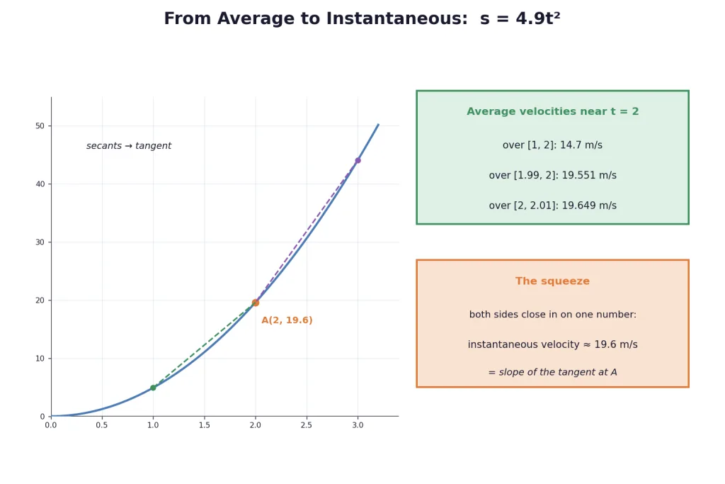
Key Point (Instantaneous velocity): the common value that average velocities approach as the interval shrinks to a point is the instantaneous velocity — geometrically, the slope of the tangent to the curve $s = 4.9t^2$ at $t = 2$. Chords tilt into the tangent; averages sharpen into an instant. This number is the derivative of $s$ at $t = 2$.

That squeezing process — "what value does the function head towards?" — deserves its own name and notation, and that is the limit.

Key Point (Limit, informally): if $f(x)$ approaches a number $l$ as $x$ approaches $a$ (from either side, without touching $a$), we write

$$\lim_{x \to a} f(x) = l$$

For example $\lim_{x \to 0} x^2 = 0$, and $h(x) = \frac{x^2 - 4}{x - 2}$ (undefined at 2) satisfies $\lim_{x \to 2} h(x) = 4$ — the values near 2 are what matter, not the value at 2.

Left-Hand and Right-Hand Limits

$x$ can approach $a$ from two directions, and each gives a one-sided limit: the left-hand limit $\lim_{x \to a^-} f(x)$ (values of $x$ below $a$) and the right-hand limit $\lim_{x \to a^+} f(x)$ (values above $a$).

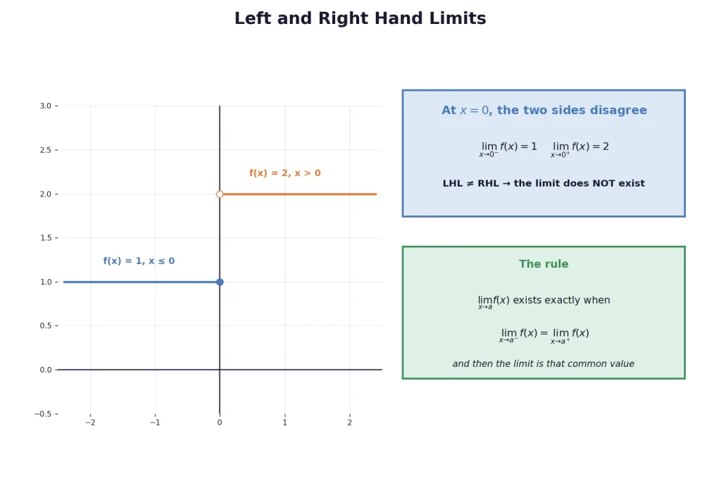
Key Point (Existence of a limit): $\lim_{x \to a} f(x)$ exists exactly when the left- and right-hand limits both exist and are equal; the limit is then that common value.

For the step function $f(x) = 1$ for $x \le 0$, $f(x) = 2$ for $x > 0$: LHL $= 1$, RHL $= 2$, so $\lim_{x \to 0} f(x)$ does not exist — even though $f(0) = 1$ is perfectly well defined.

The limit and the value are different questions. A telling example takes $f(x) = x + 2$ for $x \ne 1$ with $f(1) = 0$:

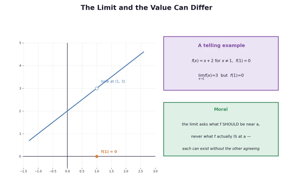
Both one-sided limits equal 3, so $\lim_{x \to 1} f(x) = 3$ — while $f(1) = 0$. Either can exist without the other, and when both exist they still need not agree.

A limit that runs away: for $f(x) = \frac{1}{x^2}$ ($x > 0$), the values exceed any bound as $x \to 0$ — written $\lim_{x \to 0} f(x) = +\infty$, a case flagged and set aside for now.

[Board Tip] For piecewise functions, always compute LHL and RHL separately using the correct branch on each side. Substituting into just one branch is the standard way to lose an existence question.

Solved Examples

Example 1: Limits by closing in

Find: (i) $\lim_{x \to 5}(x + 10)$; (ii) $\lim_{x \to 1} x^3$; (iii) $\lim_{x \to 2} 3x$.

Solution:

Step 1 — (i) Watch the values. At $x = 4.9, 4.99, 5.01$: $14.9, 14.99, 15.01$ — both sides close in on 15.

Step 2 — (ii). $0.9^3 = 0.729$, $0.99^3 \approx 0.970$, $1.01^3 \approx 1.030$: the values head to 1.

Step 3 — (iii). $3x$ heads to $3 \times 2 = 6$.

Takeaway: For these well-behaved functions the limit equals the value at the point — that is a THEOREM for polynomials, not a coincidence.

Example 2: A constant function

Find $\lim_{x \to 2} f(x)$ for $f(x) = 3$.

Solution:

Step 1 — The function never moves. Every value, at every $x$, is 3.

Step 2 — Conclude. The values near 2 are all exactly 3: $\lim_{x \to a} 3 = 3$ for every real $a$.

Takeaway: Constants pass through limits untouched — the base case every limit law builds on.

Example 3: Sums behave well

Find: (i) $\lim_{x \to 1}(x^2 + x)$; (ii) $\lim_{x \to \pi/2} \sin x$; (iii) $\lim_{x \to 0}(x + \cos x)$.

Solution:

Step 1 — (i) Split the sum. $\lim x^2 = 1$ and $\lim x = 1$: the sum's limit is $1 + 1 = 2$.

Step 2 — (ii) A trig value. $\sin x$ is continuous: the limit is $\sin\frac{\pi}{2} = 1$.

Step 3 — (iii) Mix and match. $\lim x = 0$, $\lim \cos x = \cos 0 = 1$: the sum's limit is $0 + 1 = 1$.

Takeaway: "Limit of a sum = sum of the limits" — the first limit law, already visible in numerical tables.

Example 4: One-sided limits disagree

For $f(x) = x - 2$ ($x < 0$), $f(0) = 0$, $f(x) = x + 2$ ($x > 0$), find $\lim_{x \to 0} f(x)$.

Solution:

Step 1 — LHL from the left branch. As $x \to 0^-$: $x - 2 \to -2$.

Step 2 — RHL from the right branch. As $x \to 0^+$: $x + 2 \to 2$.

Step 3 — Compare. $-2 \ne 2$: the limit does not exist — and the defined value $f(0) = 0$ cannot rescue it.

Takeaway: A defined value at the point is powerless — existence of the limit is decided by the two sides agreeing, nothing else.

Example 5: Limit exists, value differs

For $f(x) = x + 2$ ($x \ne 1$) with $f(1) = 0$, find $\lim_{x \to 1} f(x)$.

Solution:

Step 1 — Approach from both sides. For $x$ near 1 (but not equal), $f(x) = x + 2 \to 3$ from the left and from the right.

Step 2 — Conclude. LHL $=$ RHL $= 3$: $\lim_{x \to 1} f(x) = 3$.

Step 3 — Contrast with the value. $f(1) = 0 \ne 3$ — the limit serenely ignores the value planted at the point.

Takeaway: The limit asks what $f$ SHOULD be near $a$, never what it actually is at $a$.

Example 6: A two-branch check

For $f(x) = 2x + 3$ ($x \le 0$), $f(x) = 3(x + 1)$ ($x > 0$), find $\lim_{x \to 0} f(x)$ and $\lim_{x \to 1} f(x)$.

Solution:

Step 1 — At 0, both branches matter. LHL: $2x + 3 \to 3$. RHL: $3(x + 1) \to 3$.

Step 2 — They agree. $\lim_{x \to 0} f(x) = 3$.

Step 3 — At 1, only one branch is nearby. Every $x$ near 1 is positive: the limit is $3(1 + 1) = 6$.

Takeaway: Split into one-sided limits ONLY at the joining point — away from it, a single branch rules and no split is needed.

Example 7: When the branches clash

(i) $f(x) = x^2 - 1$ ($x \le 1$), $f(x) = -x^2 - 1$ ($x > 1$): find $\lim_{x \to 1} f(x)$. (ii) $f(x) = \frac{|x|}{x}$ ($x \ne 0$), $f(0) = 0$: find $\lim_{x \to 0} f(x)$.

Solution:

Step 1 — (i) Two sides. LHL: $1 - 1 = 0$; RHL: $-1 - 1 = -2$.

Step 2 — (i) Conclude. $0 \ne -2$: no limit at 1.

Step 3 — (ii) The sign function. For $x < 0$: $\frac{|x|}{x} = -1$; for $x > 0$: $+1$. LHL $= -1 \ne 1 =$ RHL — no limit.

Takeaway: $\frac{|x|}{x}$ is the canonical jump — memorise its two constant branches; it powers half the "does the limit exist" traps.

Example 8: Modulus and matched parameters

(i) Find $\lim_{x \to 5} f(x)$ for $f(x) = |x| - 5$. (ii) If $f(x) = a + bx$ ($x < 1$), $f(1) = 4$, $f(x) = b - ax$ ($x > 1$), and $\lim_{x \to 1} f(x) = f(1)$, find $a$ and $b$.

Solution:

Step 1 — (i) Resolve the modulus locally. Near 5 every $x$ is positive, so $|x| = x$: the limit is $5 - 5 = 0$.

Step 2 — (ii) Write both one-sided limits. LHL $= a + b$; RHL $= b - a$.

Step 3 — (ii) Impose the condition. Both must equal $f(1) = 4$: $a + b = 4$ and $b - a = 4$. Adding: $2b = 8$, $b = 4$; then $a = 0$.

Takeaway: A modulus is harmless once you know its sign locally; parameter-matching problems are just "set LHL = RHL = value" and solve.

Example 9: Products of factors and a two-branch split

(i) $f(x) = (x - a_1)(x - a_2)\cdots(x - a_n)$: find $\lim_{x \to a_1} f(x)$ and $\lim_{x \to a} f(x)$ for $a \ne a_i$. (ii) $f(x) = x + 1$ ($x < 0$), $f(0) = 0$, $f(x) = x - 1$ ($x > 0$): for which $a$ does $\lim_{x \to a} f(x)$ exist?

Solution:

Step 1 — (i) At a root. As $x \to a_1$ the first factor $\to 0$ while the others stay finite: the product $\to 0$.

Step 2 — (i) Away from the roots. Substitute: the limit is $(a - a_1)(a - a_2)\cdots(a - a_n)$ — a polynomial obeys $\lim =$ value.

Step 3 — (ii) Find the clash point. At 0: LHL $= 1$, RHL $= -1$ — fails. Everywhere else one branch applies: the limit exists exactly for $a \ne 0$.

Takeaway: Piecewise limits fail only where branches MEET with different values — list the joining points and test just those.

Example 10: Inferring limits

(i) If $\lim_{x \to 1} \frac{f(x) - 2}{x^2 - 1} = \pi$, find $\lim_{x \to 1} f(x)$. (ii) $f(x) = mx^2 + n$ ($x < 0$), $nx + m$ ($0 \le x \le 1$), $nx^3 + m$ ($x > 1$): when do $\lim_{x \to 0} f(x)$ and $\lim_{x \to 1} f(x)$ exist?

Solution:

Step 1 — (i) Read the structure. The quotient tends to the finite number $\pi$ while the denominator $x^2 - 1 \to 0$.

Step 2 — (i) Force the numerator down. If the numerator tended to anything non-zero, the quotient would blow up. So $f(x) - 2 \to 0$: $\lim_{x \to 1} f(x) = 2$.

Step 3 — (ii) Match at each joint. At 0: LHL $= n$, RHL $= m$ — need $m = n$. At 1: LHL $= n + m$, RHL $= n + m$ — automatic, so the limit at 1 exists for ALL $m, n$.

Takeaway: "Finite quotient over a vanishing denominator" forces the numerator to vanish too — a deduction pattern JEE reuses constantly.