Matrices — Order, Types, Equality and the Linear Operations
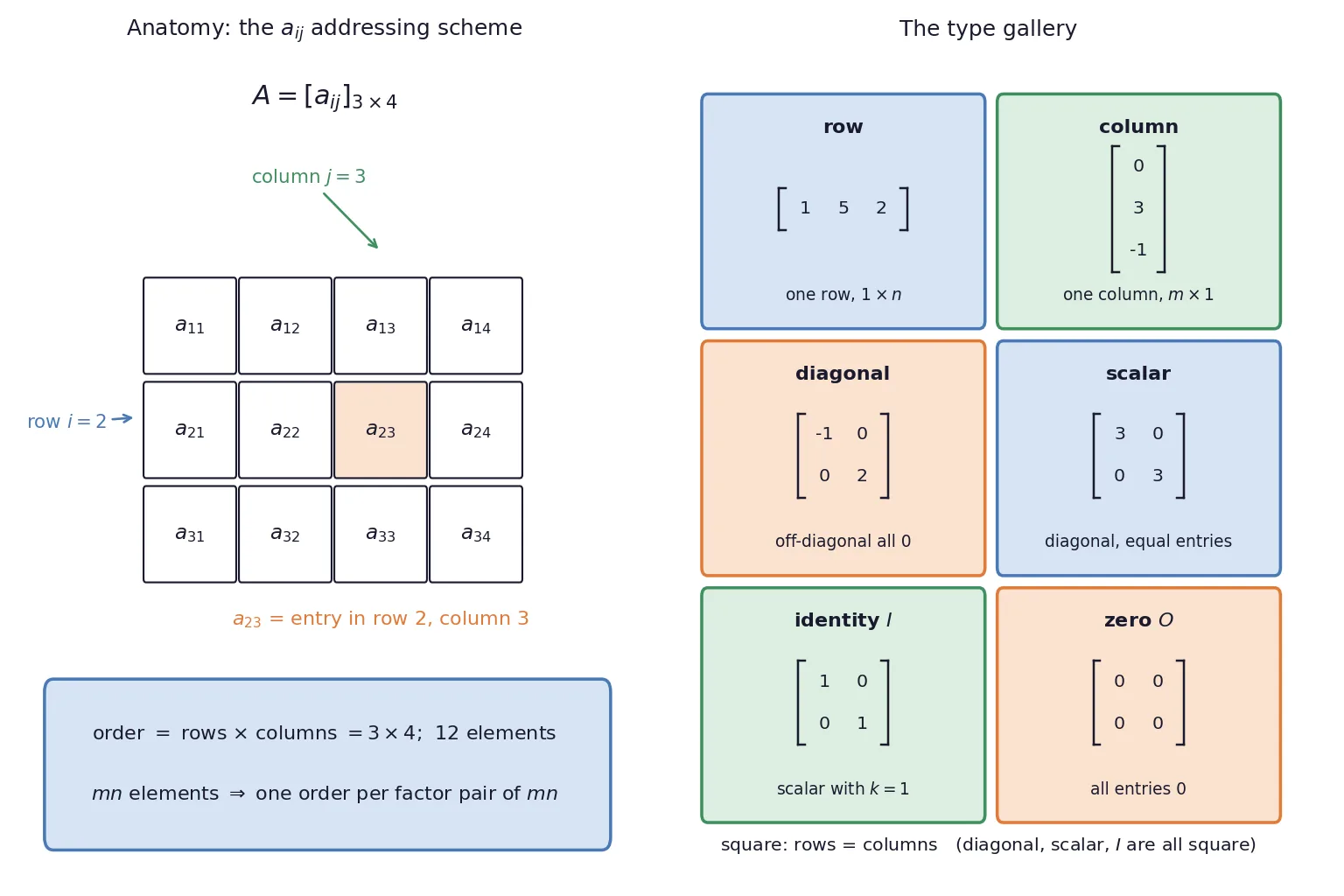
A matrix is an ordered rectangular array; with m m m n n n order is m × n m \times n m × n m n mn mn i i i j j j a i j a_{ij} a ij k k k 18 18 18 6 6 6 1 × 18 , 2 × 9 , 3 × 6 , 6 × 3 , 9 × 2 , 18 × 1 1 \times 18, 2 \times 9, 3 \times 6, 6 \times 3, 9 \times 2, 18 \times 1 1 × 18 , 2 × 9 , 3 × 6 , 6 × 3 , 9 × 2 , 18 × 1
The type gallery: row matrix (1 × n 1 \times n 1 × n m × 1 m \times 1 m × 1 m = n m = n m = n diagonal (square, a i j = 0 a_{ij} = 0 a ij = 0 scalar (diagonal with equal diagonal entries k k k k I kI k I identity I I I k = 1 k = 1 k = 1 zero matrix O O O Equality A = B A = B A = B same order and every corresponding entry equal — matching some entries is worth nothing; this is what turns matrix equations into systems of ordinary equations.
Addition and scalar multiplication
Defined entrywise, addition only for matrices of the same order . The full rulebook: A + B = B + A A + B = B + A A + B = B + A ( A + B ) + C = A + ( B + C ) (A + B) + C = A + (B + C) ( A + B ) + C = A + ( B + C ) A + O = A A + O = A A + O = A A + ( − A ) = O A + (-A) = O A + ( − A ) = O k ( A + B ) = k A + k B k(A + B) = kA + kB k ( A + B ) = k A + k B ( k + l ) A = k A + l A (k + l)A = kA + lA ( k + l ) A = k A + l A 2 A + 3 X = 5 B 2A + 3X = 5B 2 A + 3 X = 5 B X = 1 3 ( 5 B − 2 A ) X = \frac{1}{3}(5B - 2A) X = 3 1 ( 5 B − 2 A )
Multiplication — the Row-by-Column Rule and Its Surprises
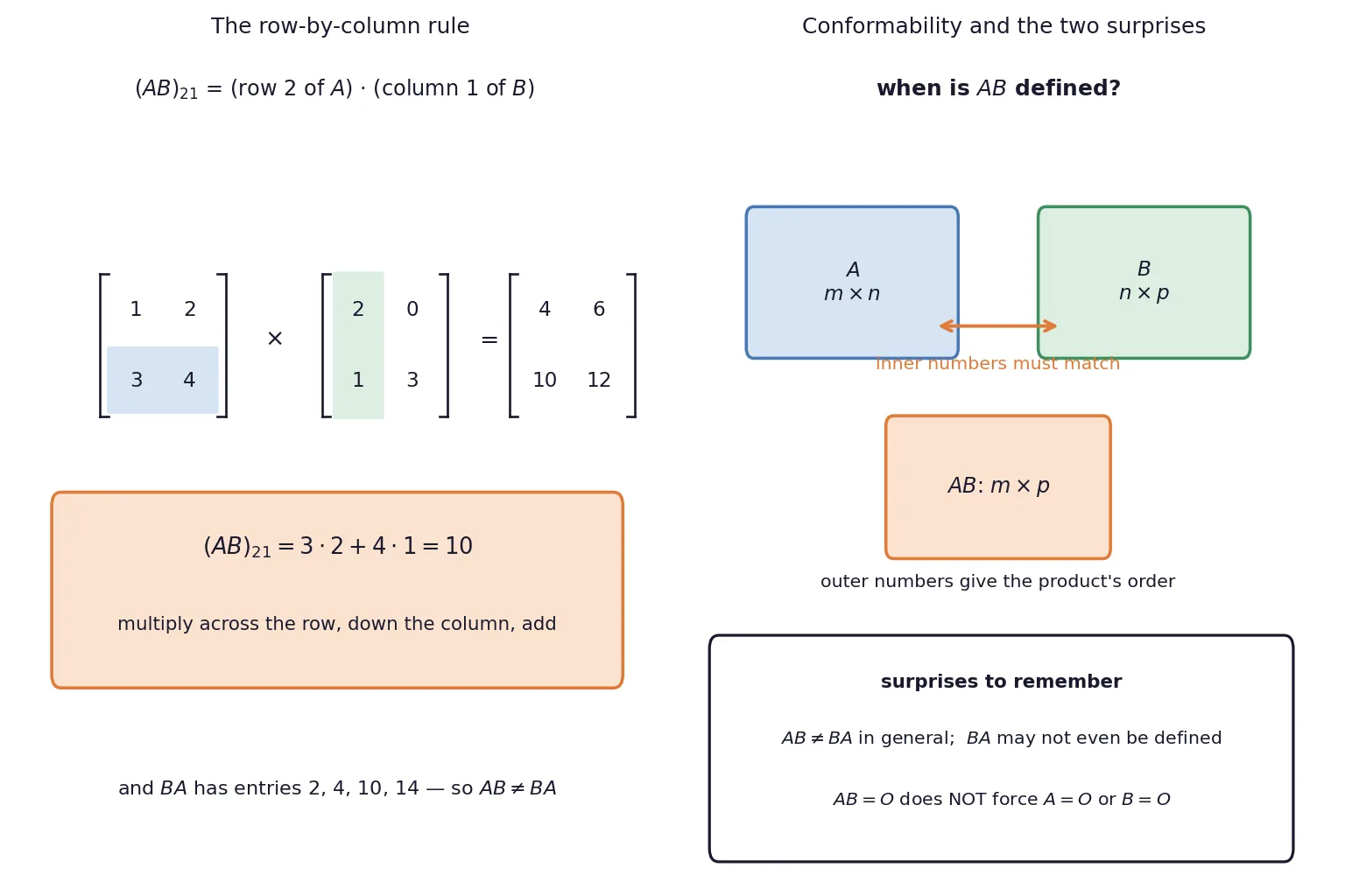
A B AB A B A A A = = = B B B m × n m \times n m × n n × p n \times p n × p m × p m \times p m × p c i k = ∑ j = 1 n a i j b j k c_{ik} = \sum_{j=1}^{n} a_{ij}b_{jk} c ik = j = 1 ∑ n a ij b j k i i i A A A k k k B B B
What survives from ordinary algebra: associativity A ( B C ) = ( A B ) C A(BC) = (AB)C A ( B C ) = ( A B ) C A I = I A = A AI = IA = A A I = I A = A breaks — the two facts every board and MCQ paper tests:
A B ≠ B A AB \neq BA A B = B A B A BA B A A B = O AB = O A B = O not force A = O A = O A = O B = O B = O B = O zero divisors exist, so a matrix factor can never be cancelled: A B = A C AB = AC A B = A C B = C B = C B = C
Transpose, Symmetric and Skew-Symmetric
A ′ A' A ′ A T A^T A T ( A ′ ) ′ = A , ( k A ) ′ = k A ′ , ( A + B ) ′ = A ′ + B ′ , ( A B ) ′ = B ′ A ′ (A')' = A, \qquad (kA)' = kA', \qquad (A + B)' = A' + B', \qquad (AB)' = B'A' ( A ′ ) ′ = A , ( k A ) ′ = k A ′ , ( A + B ) ′ = A ′ + B ′ , ( A B ) ′ = B ′ A ′ reversal in the product law is the one to memorise consciously.
Symmetric: A ′ = A A' = A A ′ = A Skew-symmetric: A ′ = − A A' = -A A ′ = − A a i i = − a i i a_{ii} = -a_{ii} a ii = − a ii 0 0 0 A A A A + A ′ A + A' A + A ′ A − A ′ A - A' A − A ′ A = 1 2 ( A + A ′ ) ⏟ symmetric + 1 2 ( A − A ′ ) ⏟ skew-symmetric \boxed{\;A = \underbrace{\tfrac{1}{2}(A + A')}_{\text{symmetric}} + \underbrace{\tfrac{1}{2}(A - A')}_{\text{skew-symmetric}}\;} A = symmetric 2 1 ( A + A ′ ) + skew-symmetric 2 1 ( A − A ′ ) uniquely into a symmetric plus a skew-symmetric part. In the exam, compute A ′ A' A ′ verify each half's property , and check the halves add back to A A A
Invertible Matrices
For square A A A B B B B B B inverse of A A A A B = B A = I AB = BA = I A B = B A = I B = A − 1 B = A^{-1} B = A − 1
Uniqueness: if B B B C C C A A A B = B I = B ( A C ) = ( B A ) C = I C = C B = BI = B(AC) = (BA)C = IC = C B = B I = B ( A C ) = ( B A ) C = I C = C Reversal: ( A B ) − 1 = B − 1 A − 1 (AB)^{-1} = B^{-1}A^{-1} ( A B ) − 1 = B − 1 A − 1 Worked Examples — Basics and Linear Operations
Example 1 — Counting possible orders
A matrix has 18 entries. What orders can it have?
Step 1 — ordered factor pairs: m n = 18 mn = 18 mn = 18 ( 1 , 18 ) , ( 2 , 9 ) , ( 3 , 6 ) , ( 6 , 3 ) , ( 9 , 2 ) , ( 18 , 1 ) (1,18), (2,9), (3,6), (6,3), (9,2), (18,1) ( 1 , 18 ) , ( 2 , 9 ) , ( 3 , 6 ) , ( 6 , 3 ) , ( 9 , 2 ) , ( 18 , 1 )
Answer: 6 6 6 3 × 6 3 \times 6 3 × 6 6 × 3 6 \times 3 6 × 3
Example 2 — Building a matrix from its rule
Construct the 2 × 2 2 \times 2 2 × 2 A = [ a i j ] A = [a_{ij}] A = [ a ij ] a i j = ( i + 2 j ) 2 2 a_{ij} = \dfrac{(i + 2j)^2}{2} a ij = 2 ( i + 2 j ) 2
Step 1 — evaluate each position: a 11 = 9 2 a_{11} = \frac{9}{2} a 11 = 2 9 a 12 = 25 2 a_{12} = \frac{25}{2} a 12 = 2 25 a 21 = 16 2 = 8 a_{21} = \frac{16}{2} = 8 a 21 = 2 16 = 8 a 22 = 36 2 = 18 a_{22} = \frac{36}{2} = 18 a 22 = 2 36 = 18
Answer: A = ( 9 2 25 2 8 18 ) A = \begin{pmatrix} \frac{9}{2} & \frac{25}{2} \\ 8 & 18 \end{pmatrix} A = ( 2 9 8 2 25 18 ) i i i j j j
Example 3 — Equality as a system of equations
Find x x x y y y ( x + 3 4 y − 2 7 ) = ( 5 4 3 7 ) \begin{pmatrix} x + 3 & 4 \\ y - 2 & 7 \end{pmatrix} = \begin{pmatrix} 5 & 4 \\ 3 & 7 \end{pmatrix} ( x + 3 y − 2 4 7 ) = ( 5 3 4 7 )
Step 1 — match entry by entry: x + 3 = 5 x + 3 = 5 x + 3 = 5 y − 2 = 3 y - 2 = 3 y − 2 = 3
Answer: x = 2 x = 2 x = 2 y = 5 y = 5 y = 5 all four had to be checked.
Example 4 — Solving a matrix equation
Find X X X X + ( 1 2 3 4 ) = ( 5 5 5 5 ) X + \begin{pmatrix} 1 & 2 \\ 3 & 4 \end{pmatrix} = \begin{pmatrix} 5 & 5 \\ 5 & 5 \end{pmatrix} X + ( 1 3 2 4 ) = ( 5 5 5 5 )
Step 1 — isolate: X = ( 5 5 5 5 ) − ( 1 2 3 4 ) X = \begin{pmatrix} 5 & 5 \\ 5 & 5 \end{pmatrix} - \begin{pmatrix} 1 & 2 \\ 3 & 4 \end{pmatrix} X = ( 5 5 5 5 ) − ( 1 3 2 4 )
Answer: X = ( 4 3 2 1 ) X = \begin{pmatrix} 4 & 3 \\ 2 & 1 \end{pmatrix} X = ( 4 2 3 1 )
Worked Examples — Multiplication
Example 5 — A B AB A B B A BA B A
For A = ( 1 2 3 4 ) A = \begin{pmatrix} 1 & 2 \\ 3 & 4 \end{pmatrix} A = ( 1 3 2 4 ) B = ( 2 0 1 3 ) B = \begin{pmatrix} 2 & 0 \\ 1 & 3 \end{pmatrix} B = ( 2 1 0 3 ) A B AB A B B A BA B A
Step 1 — row-by-column for A B AB A B ( 1 , 1 ) (1,1) ( 1 , 1 ) 1 ( 2 ) + 2 ( 1 ) = 4 1(2) + 2(1) = 4 1 ( 2 ) + 2 ( 1 ) = 4 ( 1 , 2 ) (1,2) ( 1 , 2 ) 0 + 6 = 6 0 + 6 = 6 0 + 6 = 6 ( 2 , 1 ) (2,1) ( 2 , 1 ) 6 + 4 = 10 6 + 4 = 10 6 + 4 = 10 ( 2 , 2 ) (2,2) ( 2 , 2 ) 0 + 12 = 12 0 + 12 = 12 0 + 12 = 12
Step 2 — and for B A BA B A ( 1 , 1 ) (1,1) ( 1 , 1 ) 2 ( 1 ) + 0 ( 3 ) = 2 2(1) + 0(3) = 2 2 ( 1 ) + 0 ( 3 ) = 2 ( 1 , 2 ) (1,2) ( 1 , 2 ) 4 4 4 ( 2 , 1 ) (2,1) ( 2 , 1 ) 1 + 9 = 10 1 + 9 = 10 1 + 9 = 10 ( 2 , 2 ) (2,2) ( 2 , 2 ) 2 + 12 = 14 2 + 12 = 14 2 + 12 = 14
Answer: A B = ( 4 6 10 12 ) ≠ ( 2 4 10 14 ) = B A AB = \begin{pmatrix} 4 & 6 \\ 10 & 12 \end{pmatrix} \neq \begin{pmatrix} 2 & 4 \\ 10 & 14 \end{pmatrix} = BA A B = ( 4 10 6 12 ) = ( 2 10 4 14 ) = B A
Example 6 — Zero divisors
Show that A B = O AB = O A B = O A ≠ O A \neq O A = O B ≠ O B \neq O B = O
Step 1 — the standard pair:
( 0 − 1 0 2 ) ( 3 5 0 0 ) = ( 0 0 0 0 ) \begin{pmatrix} 0 & -1 \\ 0 & 2 \end{pmatrix}\begin{pmatrix} 3 & 5 \\ 0 & 0 \end{pmatrix} = \begin{pmatrix} 0 & 0 \\ 0 & 0 \end{pmatrix} ( 0 0 − 1 2 ) ( 3 0 5 0 ) = ( 0 0 0 0 ) A A A B B B
Answer: both factors nonzero, product zero — hence cancellation of matrix factors is illegal in general.
Example 7 — A matrix satisfying a quadratic
Show that A = ( 2 0 0 3 ) A = \begin{pmatrix} 2 & 0 \\ 0 & 3 \end{pmatrix} A = ( 2 0 0 3 ) A 2 − 5 A + 6 I = O A^2 - 5A + 6I = O A 2 − 5 A + 6 I = O
Step 1 — compute the pieces: A 2 = ( 4 0 0 9 ) A^2 = \begin{pmatrix} 4 & 0 \\ 0 & 9 \end{pmatrix} A 2 = ( 4 0 0 9 ) 5 A = ( 10 0 0 15 ) 5A = \begin{pmatrix} 10 & 0 \\ 0 & 15 \end{pmatrix} 5 A = ( 10 0 0 15 ) 6 I = ( 6 0 0 6 ) 6I = \begin{pmatrix} 6 & 0 \\ 0 & 6 \end{pmatrix} 6 I = ( 6 0 0 6 )
Step 2 — combine entrywise: ( 4 − 10 + 6 , 9 − 15 + 6 ) (4 - 10 + 6, \; 9 - 15 + 6) ( 4 − 10 + 6 , 9 − 15 + 6 )
Answer: A 2 − 5 A + 6 I = O A^2 - 5A + 6I = O A 2 − 5 A + 6 I = O 2 , 3 2, 3 2 , 3 k 2 − 5 k + 6 = 0 k^2 - 5k + 6 = 0 k 2 − 5 k + 6 = 0
A A A 2 × 3 2 \times 3 2 × 3 B B B 3 × 4 3 \times 4 3 × 4 A B AB A B B A BA B A
Step 1 — A B AB A B inner dimensions 3 = 3 3 = 3 3 = 3 A B AB A B 2 × 4 2 \times 4 2 × 4
Step 2 — B A BA B A would need 4 = 2 4 = 2 4 = 2
Answer: only A B AB A B 2 × 4 2 \times 4 2 × 4 A B AB A B B A BA B A
Worked Examples — Transpose, Symmetry, Inverse
Example 9 — Verifying the reversal law
For A = ( 1 2 0 3 ) A = \begin{pmatrix} 1 & 2 \\ 0 & 3 \end{pmatrix} A = ( 1 0 2 3 ) B = ( 2 1 4 0 ) B = \begin{pmatrix} 2 & 1 \\ 4 & 0 \end{pmatrix} B = ( 2 4 1 0 ) ( A B ) ′ = B ′ A ′ (AB)' = B'A' ( A B ) ′ = B ′ A ′
Step 1 — left side: A B = ( 10 1 12 0 ) AB = \begin{pmatrix} 10 & 1 \\ 12 & 0 \end{pmatrix} A B = ( 10 12 1 0 ) ( A B ) ′ = ( 10 12 1 0 ) (AB)' = \begin{pmatrix} 10 & 12 \\ 1 & 0 \end{pmatrix} ( A B ) ′ = ( 10 1 12 0 )
Step 2 — right side: B ′ A ′ = ( 2 4 1 0 ) ( 1 0 2 3 ) = ( 10 12 1 0 ) B'A' = \begin{pmatrix} 2 & 4 \\ 1 & 0 \end{pmatrix}\begin{pmatrix} 1 & 0 \\ 2 & 3 \end{pmatrix} = \begin{pmatrix} 10 & 12 \\ 1 & 0 \end{pmatrix} B ′ A ′ = ( 2 1 4 0 ) ( 1 2 0 3 ) = ( 10 1 12 0 )
Answer: equal — and note A ′ B ′ A'B' A ′ B ′ different matrix: the reversal is essential, not cosmetic.
Example 10 — The symmetric plus skew split
Express A = ( 3 5 1 − 1 ) A = \begin{pmatrix} 3 & 5 \\ 1 & -1 \end{pmatrix} A = ( 3 1 5 − 1 )
Step 1 — transpose: A ′ = ( 3 1 5 − 1 ) A' = \begin{pmatrix} 3 & 1 \\ 5 & -1 \end{pmatrix} A ′ = ( 3 5 1 − 1 )
Step 2 — the two halves:
P = 1 2 ( A + A ′ ) = ( 3 3 3 − 1 ) , Q = 1 2 ( A − A ′ ) = ( 0 2 − 2 0 ) P = \tfrac{1}{2}(A + A') = \begin{pmatrix} 3 & 3 \\ 3 & -1 \end{pmatrix}, \qquad Q = \tfrac{1}{2}(A - A') = \begin{pmatrix} 0 & 2 \\ -2 & 0 \end{pmatrix} P = 2 1 ( A + A ′ ) = ( 3 3 3 − 1 ) , Q = 2 1 ( A − A ′ ) = ( 0 − 2 2 0 )
Step 3 — verify all three claims: P ′ = P P' = P P ′ = P Q ′ = − Q Q' = -Q Q ′ = − Q P + Q = A P + Q = A P + Q = A
Answer: A = P + Q A = P + Q A = P + Q
Example 11 — Why the halves work in general
Show that for any square matrix A A A A + A ′ A + A' A + A ′ A − A ′ A - A' A − A ′
Step 1 — transpose the sum: ( A + A ′ ) ′ = A ′ + ( A ′ ) ′ = A ′ + A = A + A ′ (A + A')' = A' + (A')' = A' + A = A + A' ( A + A ′ ) ′ = A ′ + ( A ′ ) ′ = A ′ + A = A + A ′
Step 2 — transpose the difference: ( A − A ′ ) ′ = A ′ − A = − ( A − A ′ ) (A - A')' = A' - A = -(A - A') ( A − A ′ ) ′ = A ′ − A = − ( A − A ′ )
Answer: proved in two lines from the transpose laws — this is the standard 2-mark theory question behind Example 10.
Example 12 — Verifying an inverse
Show that B = ( 2 − 3 − 1 2 ) B = \begin{pmatrix} 2 & -3 \\ -1 & 2 \end{pmatrix} B = ( 2 − 1 − 3 2 ) A = ( 2 3 1 2 ) A = \begin{pmatrix} 2 & 3 \\ 1 & 2 \end{pmatrix} A = ( 2 1 3 2 )
Step 1 — A B AB A B ( 1 , 1 ) (1,1) ( 1 , 1 ) 4 − 3 = 1 4 - 3 = 1 4 − 3 = 1 ( 1 , 2 ) (1,2) ( 1 , 2 ) − 6 + 6 = 0 -6 + 6 = 0 − 6 + 6 = 0 ( 2 , 1 ) (2,1) ( 2 , 1 ) 2 − 2 = 0 2 - 2 = 0 2 − 2 = 0 ( 2 , 2 ) (2,2) ( 2 , 2 ) − 3 + 4 = 1 -3 + 4 = 1 − 3 + 4 = 1 A B = I AB = I A B = I
Step 2 — B A BA B A the same arithmetic gives B A = I BA = I B A = I
Answer: A B = B A = I AB = BA = I A B = B A = I B = A − 1 B = A^{-1} B = A − 1 both products, and the board answer should show both.
Example 13 — Uniqueness of the inverse
Prove that if a square matrix has an inverse, it has only one.
Step 1 — suppose two: let B B B C C C A B = B A = I AB = BA = I A B = B A = I A C = C A = I AC = CA = I A C = C A = I
Step 2 — the associativity chain:
B = B I = B ( A C ) = ( B A ) C = I C = C B = BI = B(AC) = (BA)C = IC = C B = B I = B ( A C ) = ( B A ) C = I C = C
Answer: B = C B = C B = C A − 1 A^{-1} A − 1