Linear Differential Equations

The Standard Form and the Integrating Factor

A first order linear differential equation has the shape

$$\frac{dy}{dx} + P y = Q$$

where $P$ and $Q$ are constants or functions of $x$ only. Examples: $\frac{dy}{dx} + y = \sin x$; $\frac{dy}{dx} + \frac1x y = e^x$; $\frac{dy}{dx} + \frac{y}{x\log x} = \frac1x$. Note what linearity requires: $y$ and $y'$ appear to the first power, never multiplied together, never inside another function.

Where the integrating factor comes from

Multiply the equation by an unknown function $g(x)$ and demand that the left side become the derivative of the product $y\,g(x)$:

$$g(x)\frac{dy}{dx} + P\,g(x)\,y = \frac{d}{dx}\left[y\,g(x)\right] = g(x)\frac{dy}{dx} + y\,g'(x)$$

Comparing forces $P\,g(x) = g'(x)$, i.e. $\frac{g'}{g} = P$. Integrating: $\log g = \int P\,dx$, so

$$g(x) = e^{\int P\,dx} = \text{the Integrating Factor (I.F.)}$$

With it, the equation collapses to $\frac{d}{dx}\left(y\cdot\text{I.F.}\right) = Q\cdot\text{I.F.}$, and one integration finishes:

$$y\cdot(\text{I.F.}) = \int Q\cdot(\text{I.F.})\,dx + C$$

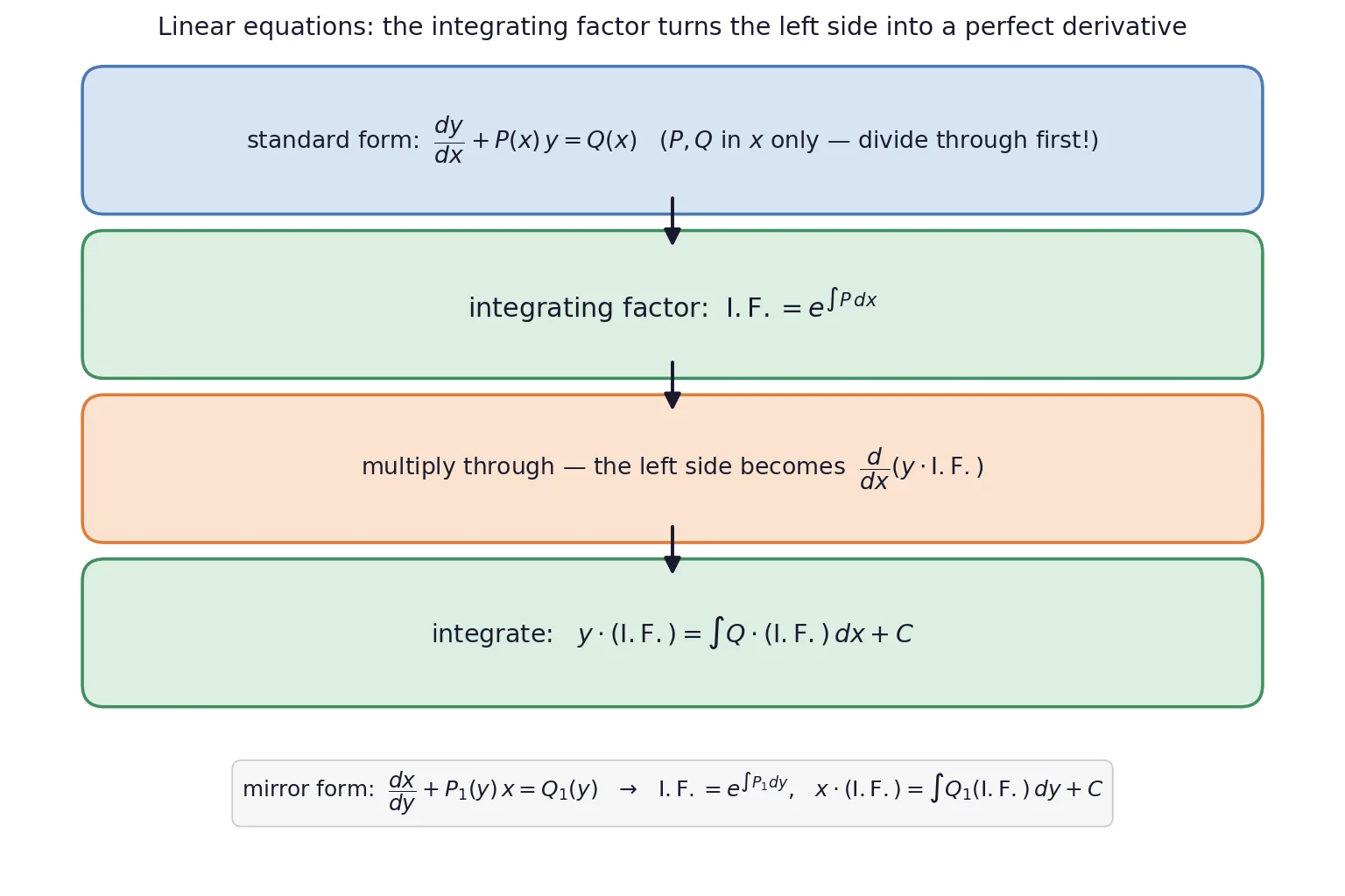
The three exam steps

1. Standardise: rewrite as $\frac{dy}{dx} + Py = Q$ — divide through by any coefficient of $\frac{dy}{dx}$ first, then read off $P$ and $Q$.
2. Compute $\text{I.F.} = e^{\int P\,dx}$ (no constant needed in this integral).
3. Write the solution $y\,(\text{I.F.}) = \int Q\,(\text{I.F.})\,dx + C$ and evaluate the right-side integral.

Key Point: The simplification $e^{\log f(x)} = f(x)$ is the daily workhorse: $P = \frac2x$ gives $\text{I.F.} = e^{2\log x} = x^2$; $P = \cot x$ gives $\text{I.F.} = e^{\log\sin x} = \sin x$; $P = -\frac1x$ gives $\frac1x$. Most integrating factors are one $\log$-collapse away.

[JEE Tip] An I.F. speed-table worth memorising: $P = \frac ax \Rightarrow \text{I.F.} = x^a$; $P = \tan x \Rightarrow \sec x$; $P = \cot x \Rightarrow \sin x$; $P = -x$-type $\Rightarrow e^{-x^2/2}$. JEE asks for the I.F. alone often enough that these four pay for themselves.

The Mirror Form — Linear in $x$

Some equations are hopeless as $\frac{dy}{dx} = \ldots$ but perfectly linear the other way round:

$$\frac{dx}{dy} + P_1 x = Q_1$$

with $P_1, Q_1$ functions of $y$ only. Then $\text{I.F.} = e^{\int P_1\,dy}$ and

$$x\cdot(\text{I.F.}) = \int Q_1\cdot(\text{I.F.})\,dy + C$$

Recognition cue: terms like $x + 2y^2$ or $x - y^2$ multiplying $dy$, with a lone $y\,dx$ — solve for $\frac{dx}{dy}$ and watch the equation become linear in $x$. Example: $y\,dx - \left(x + 2y^2\right)dy = 0$ rearranges to $\frac{dx}{dy} - \frac xy = 2y$, with $\text{I.F.} = e^{-\log y} = \frac1y$, giving $\frac xy = 2y + C$, i.e. $x = 2y^2 + Cy$.

Habits that save marks

1. Standard form before reading $P$: in $x\frac{dy}{dx} - y = 2x^2$, dividing by $x$ gives $P = -\frac1x$ (not $-1$) — the I.F. is $\frac1x$, and skipping the division is the top error on I.F. questions.
2. The right-side integral is Chapter 7: $\int Q\cdot\text{I.F.}\,dx$ routinely needs by parts ($\int e^{-x}\cos x\,dx$ loop-back), log integrals, or a lucky product-rule cancellation (as in $\int\left(2x\sin x + x^2\cos x\right)dx = x^2\sin x$).
3. Apply conditions at the very end, in the $y\cdot\text{I.F.} = \ldots + C$ form or after isolating $y$ — either is accepted.
4. Check linearity honestly: $y^2$ terms, $yy'$, or $\sin y$ mean not linear — reconsider separable or homogeneous.

Key Point: The decision tree of the chapter is now complete: product structure → separable; degree-zero ratio → homogeneous ($y = vx$); $y$ and $y'$ appearing linearly → linear (I.F.). One of the three fits every equation in the syllabus — classify first, compute second.

[JEE Tip] When both orientations look plausible, count where the nonlinearity lives: $\left(x + 3y^2\right)\frac{dy}{dx} = y$ has $y^2$ — fatal for $y$-linearity but harmless for $x$: rewrite as $\frac{dx}{dy} = \frac xy + 3y$, linear in $x$. The variable that appears only to the first power is the one to solve for.

Solved Examples

Example 1: A loop-back right side

Find the general solution of $\dfrac{dy}{dx} - y = \cos x$.

Solution:

1. Read off: $P = -1$, $Q = \cos x$; $\text{I.F.} = e^{-x}$.
2. Solution form: $ye^{-x} = \int e^{-x}\cos x\,dx + C$.
3. The by-parts loop: $\int e^{-x}\cos x\,dx = \frac{(\sin x - \cos x)e^{-x}}{2}$.
4. Isolate $y$:

Final Answer: $y = \dfrac{\sin x - \cos x}{2} + Ce^{x}$.

Example 2: Divide through first

Find the general solution of $x\dfrac{dy}{dx} + 2y = x^2$ (with $x \neq 0$).

Solution:

1. Standardise: $\frac{dy}{dx} + \frac2x y = x$, so $P = \frac2x$, $Q = x$.
2. I.F.: $e^{\int\frac2x dx} = e^{2\log x} = x^2$.
3. Solve: $y\,x^2 = \int x\cdot x^2\,dx + C = \frac{x^4}{4} + C$.

Final Answer: $y = \dfrac{x^2}{4} + Cx^{-2}$.

Example 3: Linear in $x$

Find the general solution of $y\,dx - \left(x + 2y^2\right)dy = 0$.

Solution:

1. Rearrange for $\frac{dx}{dy}$: $\frac{dx}{dy} - \frac xy = 2y$ — linear in $x$ with $P_1 = -\frac1y$, $Q_1 = 2y$.
2. I.F.: $e^{-\int\frac{dy}{y}} = e^{-\log y} = \frac1y$.
3. Solve: $x\cdot\frac1y = \int 2y\cdot\frac1y\,dy + C = 2y + C$.

Final Answer: $x = 2y^2 + Cy$.

Example 4: A cotangent coefficient with a condition

Find the particular solution of $\dfrac{dy}{dx} + y\cot x = 2x + x^2\cot x$ (with $x \neq 0$), given $y = 0$ when $x = \frac{\pi}{2}$.

Solution:

1. I.F.: $e^{\int\cot x\,dx} = e^{\log\sin x} = \sin x$.
2. Solve: $y\sin x = \int\left(2x\sin x + x^2\cos x\right)dx + C$ — the integrand is exactly $\frac{d}{dx}\left(x^2\sin x\right)$, so $y\sin x = x^2\sin x + C$.
3. Apply the condition: $0 = \frac{\pi^2}{4}\cdot1 + C$, so $C = -\frac{\pi^2}{4}$.

Final Answer: $y\sin x = x^2\sin x - \dfrac{\pi^2}{4}$, i.e. $y = x^2 - \dfrac{\pi^2}{4\sin x}$ (for $\sin x \neq 0$).

Takeaway: Before grinding $\int Q\cdot\text{I.F.}\,dx$ by parts, check whether the integrand is a ready-made product-rule derivative — exam setters plant these gifts deliberately.

Example 5: A curve through a point

Find the equation of the curve through $(0, 1)$ whose tangent slope at $(x, y)$ equals the sum of the abscissa and the product of abscissa and ordinate.

Solution:

1. Translate: $\frac{dy}{dx} = x + xy$, i.e. $\frac{dy}{dx} - xy = x$ — linear with $P = -x$, $Q = x$.
2. I.F.: $e^{\int(-x)dx} = e^{-x^2/2}$.
3. Solve: $ye^{-x^2/2} = \int xe^{-x^2/2}dx + C = -e^{-x^2/2} + C$ (substitute $t = -\frac{x^2}{2}$).
4. Isolate and apply $(0, 1)$: $y = -1 + Ce^{x^2/2}$; $1 = -1 + C$ gives $C = 2$.

Final Answer: $y = 2e^{x^2/2} - 1$.

Example 6: The cleanest I.F. exercise

Find the general solution of $\dfrac{dy}{dx} + \dfrac{y}{x} = x^2$.

Solution:

1. Read off: $P = \frac1x$; $\text{I.F.} = e^{\log x} = x$.
2. Solve: $yx = \int x\cdot x^2\,dx + C = \frac{x^4}{4} + C$.

Final Answer: $xy = \dfrac{x^4}{4} + C$.

Example 7: Tangent coefficient with a condition

Find the particular solution of $\dfrac{dy}{dx} + 2y\tan x = \sin x$, given $y = 0$ when $x = \frac{\pi}{3}$.

Solution:

1. I.F.: $e^{2\int\tan x\,dx} = e^{2\log\sec x} = \sec^2x$.
2. Solve: $y\sec^2x = \int\sin x\sec^2x\,dx + C = \int\sec x\tan x\,dx + C = \sec x + C$.
3. Apply the condition: at $x = \frac{\pi}{3}$: $0 = \sec\frac{\pi}{3} + C = 2 + C$, so $C = -2$.
4. Isolate: $y = \cos x - 2\cos^2x$.

Final Answer: $y = \cos x - 2\cos^2 x$.

Takeaway: $e^{2\log\sec x} = \sec^2x$ — the log-collapse works with any coefficient: $e^{a\log f} = f^a$. Squares and reciprocals of the speed-table entries appear constantly.