Quick Revision

Mean of a List

• Mean $= \frac{\text{sum}}{\text{count}}$, so the sum is the mean times the count.
• Values in equal steps: mean $= \frac{\text{first} + \text{last}}{2}$.
• First $n$ natural numbers: $\frac{n + 1}{2}$; first $n$ even: $n + 1$; first $n$ odd: $n$.
• Squares of 1 to $n$: $\frac{(n + 1)(2n + 1)}{6}$.
• Working mean $A$: $\bar{x} = A + \frac{\sum d}{n}$, where $d = x - A$.
• Deviations from the mean add up to 0.

For example: the mean of 6, 9, 12, …, 60 is $\frac{6 + 60}{2} = 33$.

When the Values Change

• A wrong value corrected: the mean changes by $\frac{\text{correct value} - \text{wrong value}}{n}$.
• A value added or removed: find the new total and divide by the new count.
• Add $k$ to every value: the mean, median and mode go up by $k$. Multiply by $k$: they are multiplied by $k$. So $y = ax + b$ gives $\bar{y} = a\bar{x} + b$.

For example: 10 values have mean 18, but 27 was read as 72. The mean falls by $\frac{45}{10} = 4.5$, to 13.5. Word problems on averages are in Chapter 5.

Weighted and Combined Mean

• Weighted mean $= \frac{\sum wx}{\sum w}$.
• Combined mean of groups $= \frac{n_1\bar{x}_1 + n_2\bar{x}_2 + n_3\bar{x}_3}{n_1 + n_2 + n_3}$.
• It lies between the group means, nearer to the mean of the bigger group.
• Two groups with combined mean $M$: $n_1 : n_2 = (\bar{x}_2 - M) : (M - \bar{x}_1)$.
• The plain average of the group means works only for groups of equal size.

For example: 25 men with mean age 40 and 15 women with mean age 32: $\frac{1000 + 480}{40} = 37$ years, not 36.

Mean of a Frequency Table

• Discrete table: $\bar{x} = \frac{\sum fx}{\sum f}$.
• Grouped table: use class marks, $x = \frac{\text{lower limit} + \text{upper limit}}{2}$.
• Assumed mean: $\bar{x} = A + \frac{\sum fd}{\sum f}$, with $d = x - A$.
• Step deviation: $u = \frac{x - A}{h}$ and $\bar{x} = A + h \times \frac{\sum fu}{\sum f}$.
• A missing frequency: use $\sum f(x - \bar{x}) = 0$, or put $A$ at the value whose frequency is missing.
• The plain mean of the class marks, without the frequencies, is not the mean of the table.

Median of a List and a Discrete Table

• Arrange the values in order first.
• $n$ odd: the median is the $\frac{n + 1}{2}$-th value. $n$ even: it is the mean of the $\frac{n}{2}$-th and the $\left(\frac{n}{2} + 1\right)$-th values.
• Discrete table: write the cumulative frequencies and see where those positions fall.
• The two middle values can fall in different rows; then the median is their mean.

For example: 9, 4, 15, 7, 12, 4 in order is 4, 4, 7, 9, 12, 15, so the median is $\frac{7 + 9}{2} = 8$.

Median of Grouped Data

$$\text{Median} = L + \frac{\frac{N}{2} - cf}{f} \times h$$

• The median class is the first class whose cumulative frequency reaches $\frac{N}{2}$.
• $cf$ belongs to the class before the median class.
• Inclusive classes (10-19, 20-29) first become 9.5-19.5, 19.5-29.5.
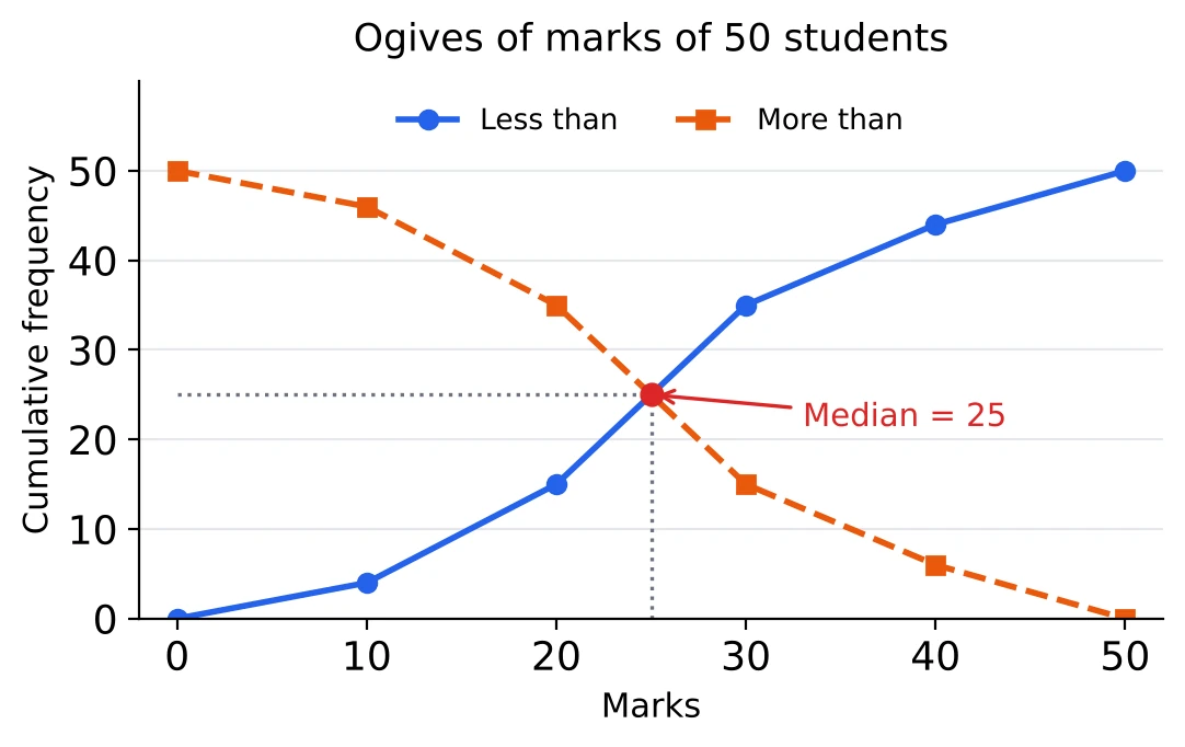
• 'Less than' figures are already cumulative; 'more than' figures give class frequencies by subtraction.
• The 'less than' and 'more than' ogives cross at the median, where each reaches $\frac{N}{2}$.

Quartiles

• Lower quartile $Q_1$: the $\frac{n + 1}{4}$-th value in order.
• Upper quartile $Q_3$: the $\frac{3(n + 1)}{4}$-th value in order.
• The median is the middle quartile, $Q_2$.
• Interquartile range $= Q_3 - Q_1$. It is the spread of the middle half of the data, so extreme values do not affect it.

For example: for 3, 5, 6, 8, 10, 11, 13 ($n = 7$), $Q_1$ is the 2nd value, 5, the median is 8, and $Q_3$ is the 6th value, 11. The interquartile range is $11 - 5 = 6$.

Mode

• The mode is the value that occurs most often. A list can have one mode, two modes, or none when every value occurs once.
• Discrete table: the value with the highest frequency.
• Grouped data: $\text{Mode} = L + \frac{f_1 - f_0}{2f_1 - f_0 - f_2} \times h$, with $f_1$ for the modal class and $f_0$, $f_2$ for the classes before and after it.
• The mode leans towards the bigger neighbour; when $f_0 = f_2$, it is the middle of the class.
• If the modal class is the first class, $f_0 = 0$.

Empirical Relation and Choosing an Average

• $\text{Mode} = 3\,\text{Median} - 2\,\text{Mean}$ for moderately skewed data; also $\text{Mean} - \text{Mode} = 3(\text{Mean} - \text{Median})$.
• Symmetric data: mean, median and mode are equal.
• A long tail of high values: $\text{Mode} < \text{Median} < \text{Mean}$. A long tail of low values: the order is reversed.
• The mode suits the most common size (shoes, shirts); the median suits data with a few extreme values (incomes); the mean uses every value.

For example: mean 40 and median 38 give $\text{Mode} = 114 - 80 = 34$.

Range and Mean Deviation

• Range $=$ largest value $-$ smallest value.
• Coefficient of range $= \frac{\text{largest} - \text{smallest}}{\text{largest} + \text{smallest}}$.
• Mean deviation about the mean $= \frac{\sum \lvert x - \bar{x} \rvert}{n}$. About the median, use the median in place of $\bar{x}$.
• Mean deviation adds distances, so all the signs are dropped.

For example: for 4, 6, 9, 13, 18, the range is 14 and the coefficient of range is $\frac{14}{22} \approx 0.64$. The mean is 10, the distances from it are 6, 4, 1, 3, 8, and the mean deviation is $\frac{22}{5} = 4.4$.

Variance and Standard Deviation

• $\sigma^2 = \frac{\sum (x - \bar{x})^2}{n} = \frac{\sum x^2}{n} - \bar{x}^2$, and $\sigma = \sqrt{\sigma^2}$.
• Frequency table: $\sigma^2 = \frac{\sum fx^2}{\sum f} - \bar{x}^2$.
• With $u = \frac{x - A}{h}$: $\sigma^2 = h^2\left[\frac{\sum fu^2}{\sum f} - \left(\frac{\sum fu}{\sum f}\right)^2\right]$.
• Two values $a$ and $b$: $\sigma = \frac{\lvert a - b \rvert}{2}$.
• First $n$ natural numbers: $\sigma^2 = \frac{n^2 - 1}{12}$.
• $\sigma$ is never negative, and it is 0 only when all the values are equal.

Changes and the Coefficient of Variation

• Adding or subtracting $k$: the variance and the SD do not change.
• Multiplying by $k$: the SD is multiplied by $\lvert k \rvert$ and the variance by $k^2$.
• $\text{CV} = \frac{\sigma}{\bar{x}} \times 100$. The smaller CV belongs to the more consistent data.
• SDs alone can be compared only when the means are equal.

For example: marks with SD 3, doubled and then raised by 5, have SD 6 and variance 36. Mean 50 with SD 5 (CV 10%) is more consistent than mean 30 with SD 4.5 (CV 15%).

Before the Exam

Mistakes to watch for:

• the median of a list taken before sorting;
• $\frac{N + 1}{2}$ used for grouped data;
• the cf of the median class used in place of the class before;
• $f_0$ and $f_2$ swapped, or $h$ left out;
• $3\,\text{Mean} - 2\,\text{Median}$ written for the mode;
• the variance given when the SD is asked;
• the SD changed by adding a constant, or $k$ used for $k^2$;
• inclusive classes not made continuous.

Chapter Test: 25 questions in 25 minutes; $+3$ right, $-1$ wrong.