
Reading a Line Graph
A line graph shows how one quantity changes, usually over time. The years (or months) run along the horizontal axis and the values go up the vertical axis. Each value is marked with a point, and the points are joined in order by straight lines.
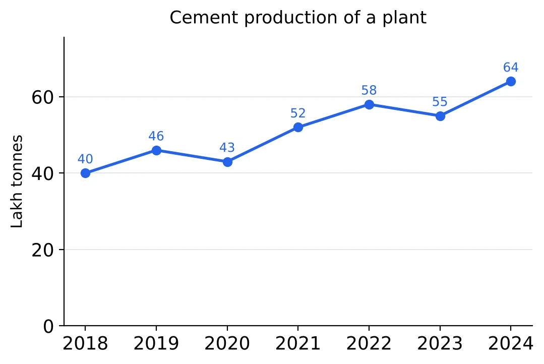
- The highest point is 2024 (64 lakh tonnes) and the lowest is 2018 (40 lakh tonnes).
- A segment going up means the value rose from one year to the next; a segment going down means it fell. Production fell in 2020 and in 2023 and rose in the other four years.
- The points are the data. The lines between them only guide the eye. The graph does not tell you what happened in the middle of 2020, so never read a value off a line between two points.
Reading the values. When the values are printed at the points, use them. When they are not, go straight across from the point to the vertical scale, and check what one gap between grid lines is worth before you read anything: on a scale marked 0, 10, 20, the small gaps may be 2 or 5.
Number of years with a rise. Count the rising segments: 2019, 2021, 2022 and 2024, so production rose in 4 years. A segment belongs to the later of its two years: 'rose in 2021' means from 2020 to 2021. The first year, 2018, has nothing before it, so it is never counted as a rise or a fall.
Total over a period. Add the points: from 2021 to 2023 the plant produced lakh tonnes.
Comparing two years. Production in 2024 was times that of 2018, so the ratio of 2018 to 2024 is 5 : 8.
Units. The scale says lakh tonnes. If the options are written in tonnes, 64 lakh tonnes is 64,00,000 tonnes; check the unit of the options before you compare numbers.
Increase, Decrease and the Steepest Rise
On a line graph the years are equally spaced, so the steepness of a segment shows the size of the change: the steeper the segment, the bigger the rise or fall in actual numbers.
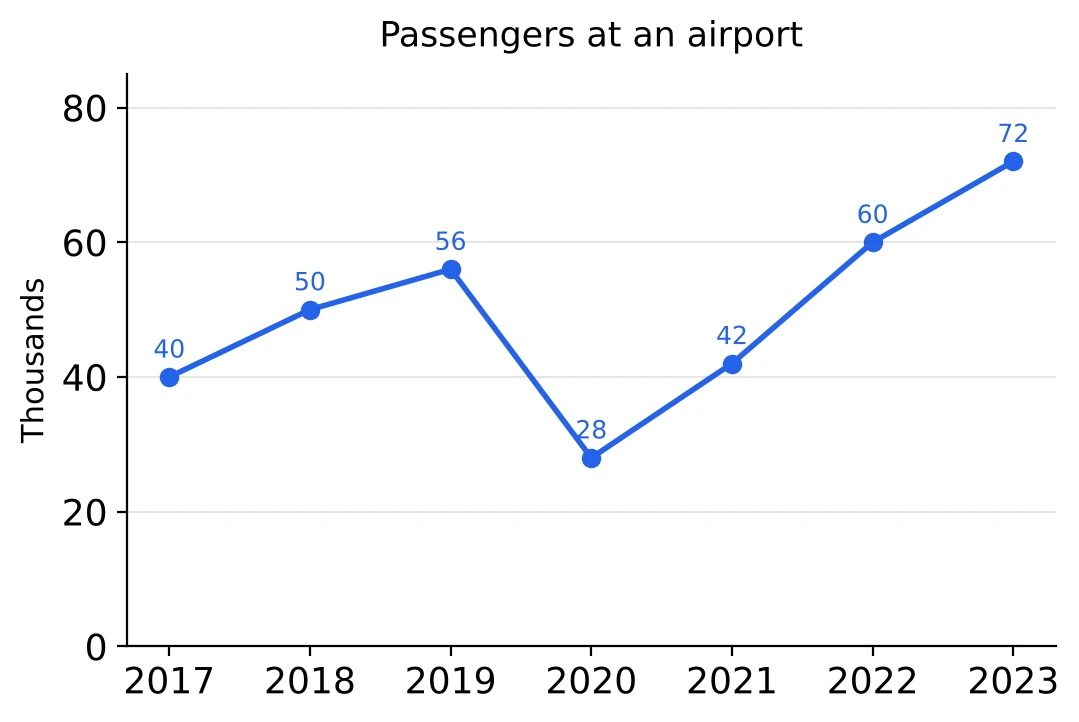
| Year | 2018 | 2019 | 2020 | 2021 | 2022 | 2023 |
|---|---|---|---|---|---|---|
| Change from the year before (thousand) | ||||||
| Percentage change | 25% | 12% | 50% | 20% |
- Steepest rise: from 2021 to 2022, by 18 thousand.
- Steepest fall: from 2019 to 2020, by 28 thousand.
- Largest percentage rise: from 2020 to 2021, 50%. That is not the steepest segment: a rise of 14 on a low base of 28 is a bigger percentage than a rise of 18 on 42.
So 'the greatest increase' and 'the greatest percentage increase' can be different years. Read which one the question asks for.
The base is always the earlier year, whether the line goes up or down (see Chapter 3). From 2019 to 2020 the fall is ; dividing by 28 instead would give 100%, which would mean the airport had no passengers at all.
A fall and an equal percentage rise do not cancel. Passengers fell by 50% in 2020 (56 to 28) and rose by 50% in 2021 (28 to 42), but 42 is still below 56. The first year after 2019 with more passengers than 2019 is 2022.
Finding the largest percentage change quickly. You need not work out every percentage. A large rise on a small base wins, so compare only the likely ones as fractions: against . Since is bigger, 2021 has the larger percentage rise.
Totals and Averages from a Line Graph
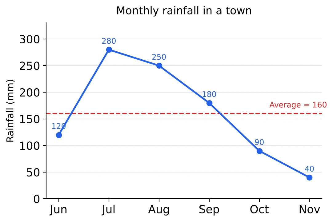
The average of a line graph is the total of its points divided by the number of points. The town's rainfall from June to November was
over 6 months, so the average is mm a month. The dashed line marks it. July, August and September lie above it; the other three months lie below.
Faster adding with a working value. Pick a round number near the middle, say 150, and add only the differences from it: . Shared over 6 months that is 10, so the average is . The differences are small numbers, which keeps the mental arithmetic short (the method is in Chapter 5).
The average of part of the graph. From July to September: mm. Count the points carefully: July to September is three months, not two.
A missing value from an average. Suppose you are also told that the average from June to December was 140 mm. Then the seven months had mm in all, and December had mm.
Months above the average. First find the average, then count the points above it: here 3. Answering from the look of the graph is risky when a point is close to the average line, so compare the numbers.
Share of the total. July and August together brought of the season's rain.
Multiple Line Graphs
When two or three quantities are drawn on one graph, each has its own line, told apart by colour, marker and line style, with a legend that says which is which. Read the legend first. Reading the right year off the wrong line is an easy mistake when the lines run close together.
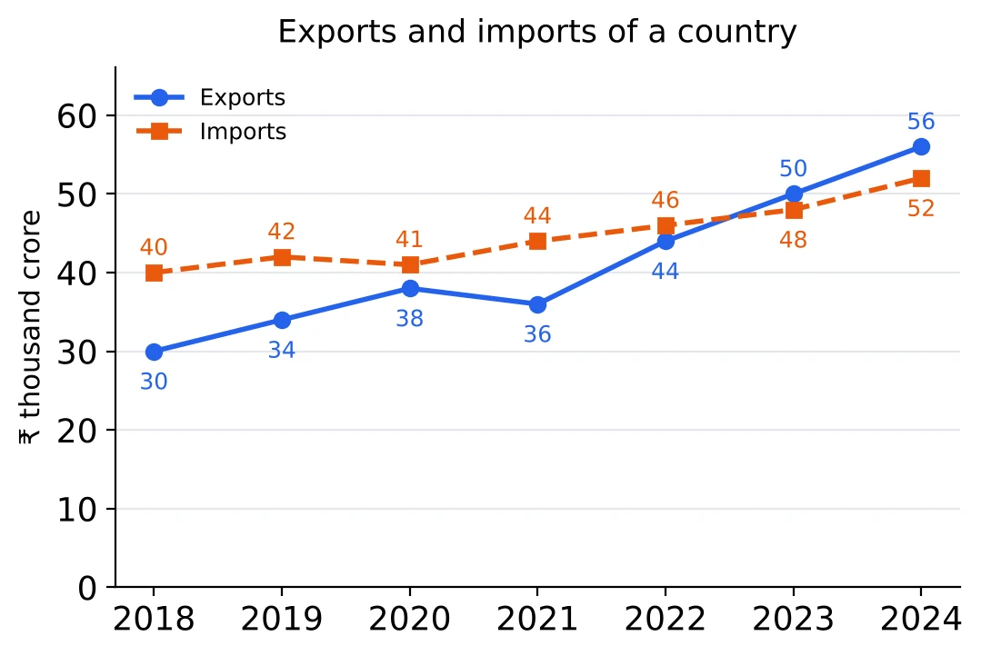
The gap between the lines is the difference of the two quantities in that year. Imports minus exports was 10 in 2018, 8 in 2019, 3 in 2020, 8 in 2021 and 2 in 2022 (all in ₹ thousand crore). The gap was widest in 2018.
Where the lines cross. The lines cross between 2022 and 2023: in 2022 imports were higher (46 against 44), and in 2023 exports were higher (50 against 48). So 2023 is the first year in which exports were more than imports. The crossing point itself is not a data value; a question about it is really asking in which year the order first changed.
A ratio or a percentage in one year. In 2020, exports : imports = 38 : 41. In 2024, exports were of imports.
Comparing the growth of the two. From 2018 to 2024, exports rose by and imports by . Be careful with steepness here. Two lines that rise by the same amount look equally steep, but the one that starts lower has grown by the larger percentage.
A total of the two lines. Total trade (exports plus imports) in 2022 was thousand crore rupees.
[SSC Tip] For 'in how many years was A more than B', put a small tick against each year as you check it and count the ticks. With seven years and two lines it is easy to miss a year where the points are close.
Line Graphs That Show Percentages
Some line graphs show a percentage for each year, not an amount: percentage profit, growth rate, pass percentage. The line then tells you about rates only, and you need one more amount from the question to find any amount.
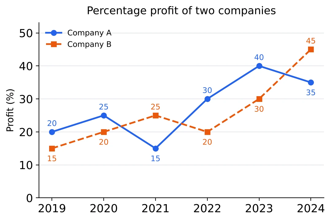
Percentage profit.
- A spent ₹ 60 crore in 2022, when its profit was 30%. Its income was , that is ₹ 78 crore.
- B's income in 2021 was ₹ 75 crore, at a profit of 25%. Its expenditure was , that is ₹ 60 crore. Taking 25% off 75 gives 56.25, which is wrong, because the profit percentage is worked on the expenditure, not on the income.
- If A and B had equal incomes in 2023, their expenditures were in the ratio , that is . The company with the higher profit percentage spent less.
What the graph cannot tell you. It does not say which company made more profit in rupees, or whether A's profit in rupees fell in 2024. A's percentage fell from 40% to 35%, but if A spent much more in 2024, its profit in rupees could still have gone up. When a question asks for an amount and no amount is given, 'cannot be determined' may well be the right option.
Growth-rate graphs. If the line shows the percentage increase over the previous year, a falling line that stays above 0 still means growth, only slower growth. The value itself goes down only in a year when the rate is below 0. Rates multiply over the years: growth of 10% and then 20% gives , a total rise of 32%, not 30%.
Histograms
A histogram shows a frequency distribution: how many items fall in each class interval. It looks like a bar graph, with three differences.
- The horizontal axis is a continuous scale (marks, heights, ages), and each bar stands on its class interval.
- The bars touch, because each class ends where the next one begins.
- The width of a bar is the class width. When all classes have the same width, the height of a bar is its frequency.
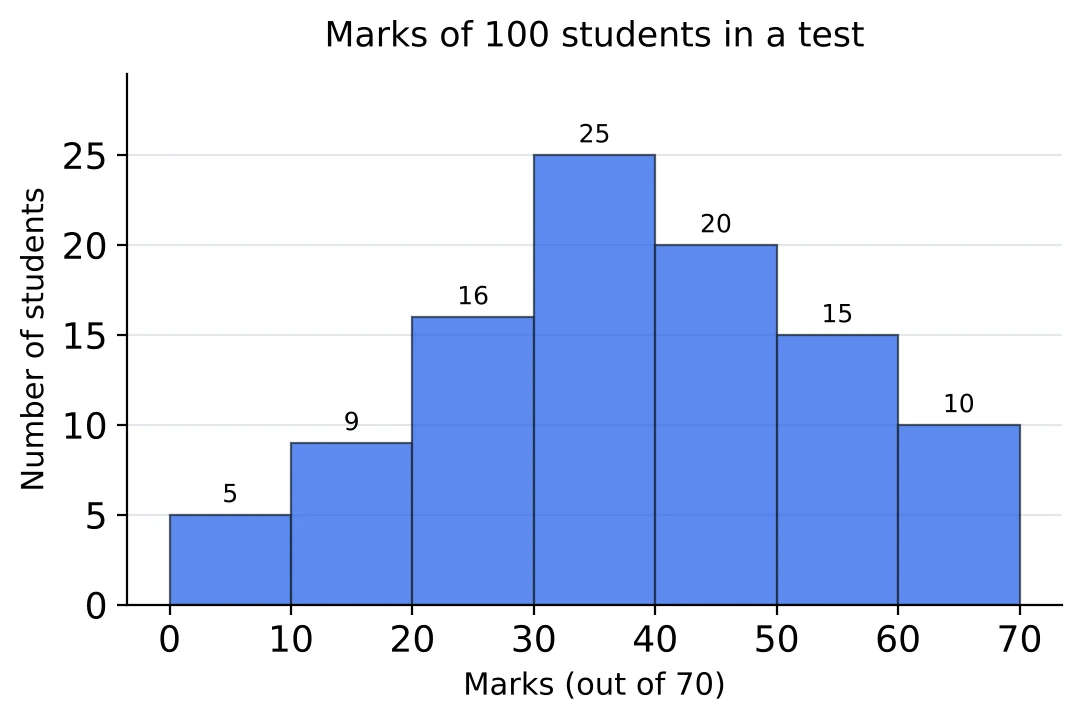
Class intervals. The class 30-40 holds marks from 30 up to, but not including, 40. A student who scored exactly 40 is counted in 40-50. For this class the lower limit is 30, the upper limit is 40 and the class width is 10.
Reading the histogram.
- The class with the highest frequency is 30-40, with 25 students.
- Total number of students: .
- Scored less than 20: .
- Scored at least 40, that is 40 or more: .
- Scored 20 or more but less than 50: .
- Percentage who scored 50 or more: .
'At least' and 'less than'. 'At least 40' starts with the bar that begins at 40. 'Less than 40' stops with the bar that ends at 40. Find that edge on the axis before you add: one bar too many or too few gives a wrong option that looks quite reasonable.
Using the complement. 'At least 40' is also the total minus 'less than 40': . When most of the bars lie on one side, add the few on the other side and subtract from the total.
Working out the mean, median and mode of such a distribution is the subject of Chapter 19; here we only read the chart.
A Histogram from a Table, and a Table from a Histogram
Drawing a histogram from a table. Mark the class limits on the horizontal axis and draw a bar over each class, as tall as its frequency. With classes like 0-10, 10-20, where each class ends where the next begins, you can draw straight away.
Tables of ages, counts or scores may be written with gaps instead: 20-24, 25-29, 30-34. These are inclusive classes, where a person aged 24 is in the first class and one aged 25 is in the second. A histogram cannot have gaps, so first make the classes continuous. The gap between 24 and 25 is 1, so take half of it, 0.5, away from every lower limit and add 0.5 to every upper limit.
| Age (years) | 20-24 | 25-29 | 30-34 | 35-39 | 40-44 | 45-49 |
|---|---|---|---|---|---|---|
| Class boundaries | 19.5-24.5 | 24.5-29.5 | 29.5-34.5 | 34.5-39.5 | 39.5-44.5 | 44.5-49.5 |
| Employees | 12 | 26 | 32 | 24 | 16 | 10 |
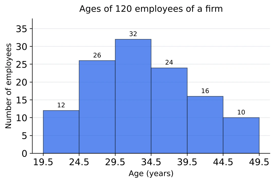
The bars now stand on 19.5-24.5, 24.5-29.5 and so on, and they touch. The class width is 5, from 19.5 to 24.5, not 4. The axis does not start at 0, which is normal for a histogram whose first class starts far from 0.
Reading a table back from a histogram. Go along the bars from left to right and write each class with its bar height. If the axis shows boundaries such as 29.5 and 34.5, the class in the original table was 30-34. From this histogram:
- employees aged 30 to 34: 32;
- employees aged 40 or more: ;
- employees under 30: , which is of the staff.
Bars labelled by class marks. Some histograms print the middle value of each class under its bar instead of the edges: 22, 27, 32 and so on. The middle value is the class mark, . Each class then runs from half a width below its mark to half a width above it; with marks 5 apart, the mark 32 stands for 29.5 to 34.5, the class 30-34 of the table.
Cumulative Frequency: Less Than and At Least
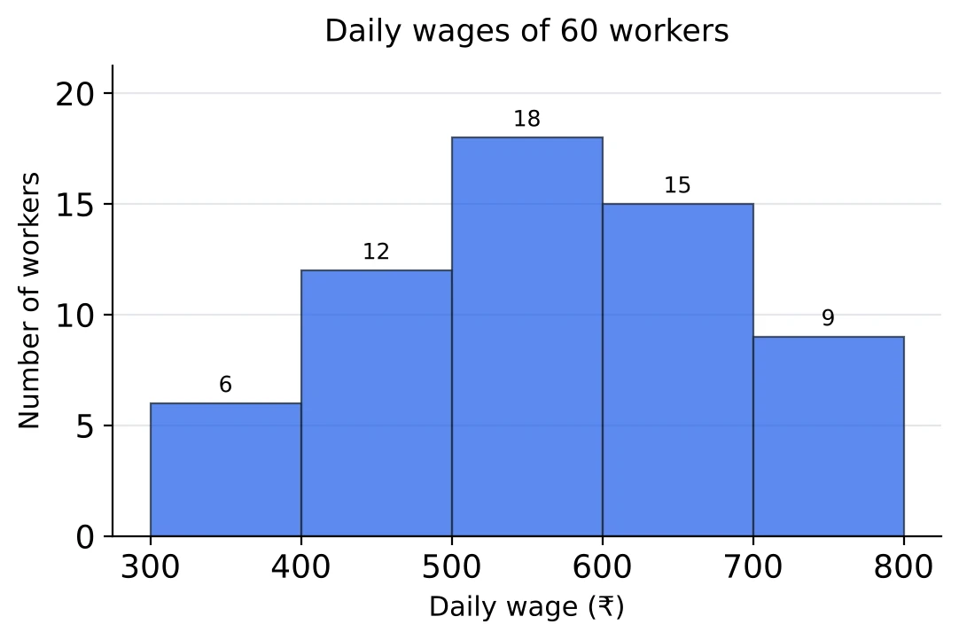
Questions like 'how many workers earn less than ₹ 600 a day?' need running totals. Add the bars from the left to get a less-than row, and from the right to get an at-least row:
| Daily wage (₹) | 300-400 | 400-500 | 500-600 | 600-700 | 700-800 |
|---|---|---|---|---|---|
| Workers | 6 | 12 | 18 | 15 | 9 |
| Less than the upper limit | 6 | 18 | 36 | 51 | 60 |
| At least the lower limit | 60 | 54 | 42 | 24 | 9 |
So 36 workers earn less than ₹ 600 and 24 earn at least ₹ 600. The two always add up to the total, 60, which is a quick check on your adding.
A range in the middle. Workers earning at least ₹ 500 but less than ₹ 700: . From the less-than row the same number is .
Back from a cumulative row to the classes. Suppose you are given only the less-than row 6, 18, 36, 51, 60. Subtract each entry from the next one: , , and . The first class keeps its own value, 6. These are the heights of the histogram's bars, so the histogram can be drawn from a cumulative table. Cumulative tables on their own are taken up in Tables.
Percentages. The percentage of workers earning at least ₹ 600 is .
Watch the words. 'Less than 600' leaves out the class 600-700 completely, because a wage of exactly ₹ 600 belongs to that class. 'More than 600' is read from the 600-700 class onwards, the same as 'at least 600': the table cannot separate the workers who earn exactly ₹ 600, so questions treat the two alike.
Frequency Polygons
A frequency polygon shows the same distribution as a histogram, with a line in place of bars. To draw it over a histogram:
- Mark the mid-point of the top of each bar. Its position on the horizontal axis is the class mark, .
- Join these points in order with straight lines.
- Close the polygon at both ends. Take an empty class (frequency 0) before the first class and another after the last, and join the line down to their class marks on the horizontal axis.
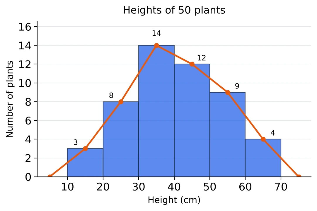
Here the class marks are 15, 25, 35, 45, 55 and 65. The empty class before 10-20 is 0-10, with mark 5, and the one after 60-70 is 70-80, with mark 75. So the polygon starts at and ends at .
Reading the polygon. Each corner of the polygon is one class: its height is the frequency and its position is the class mark. The highest corner, 14 at the mark 35, tells you that the class 30-40 has the most plants. The two end points on the axis are not classes; they only close the figure.
Why close it? Closed this way, the polygon encloses the same area as the histogram. Each small triangle the line cuts off a bar is matched by an equal triangle it adds outside the bars. So the polygon and the histogram stand for the same total, 50 plants.
Changes between classes. The steepest rise of the polygon is from the mark 25 to the mark 35, from 8 to 14 plants (up 6). The steepest fall is from 55 to 65, from 9 to 4 plants (down 5). As with a line graph, steepness shows the size of the change because the classes are equally wide.
Reading a Frequency Polygon on Its Own; Comparing Two
A frequency polygon can be drawn without the histogram, with only the class marks on the horizontal axis. To get the classes back:
- the class width is the gap between two neighbouring marks, here ;
- each class runs from half a width below its mark to half a width above it, so the mark 45 means the class 40-50.
The two end points on the axis (15 and 85 here) are the closing points and carry frequency 0.
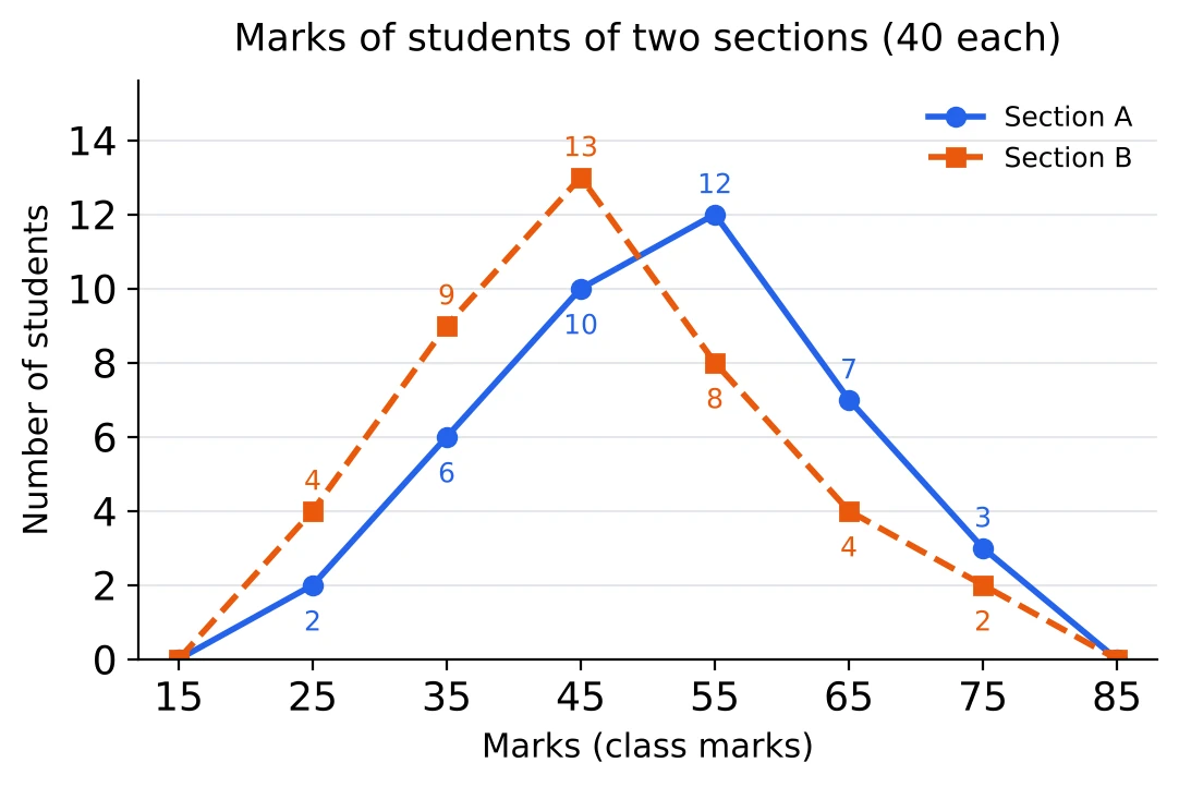
The graph shows the marks of 40 students in each of two sections. Reading both polygons gives this table:
| Marks | 20-30 | 30-40 | 40-50 | 50-60 | 60-70 | 70-80 |
|---|---|---|---|---|---|---|
| Section A | 2 | 6 | 10 | 12 | 7 | 3 |
| Section B | 4 | 9 | 13 | 8 | 4 | 2 |
- Students with 50 marks or more: A , B .
- Students with less than 40: A , B .
- The polygons cross between the marks 45 and 55. Up to the class 40-50, B has more students in each class; from 50-60 onwards, A has more. A's polygon sits further to the right, so Section A did better.
- The gap between the sections is largest in the class 50-60: students.
Both sections have 40 students, so comparing the counts is fair. If the two groups were of different sizes, you would compare percentages instead.
Two polygons on one pair of axes are easier to compare than two histograms, which would hide each other. That is the main use of a frequency polygon.
[Tier 2] Unequal Class Widths and Frequency Density
When the classes are not all the same width, bars as tall as the frequencies would mislead. A class twice as wide collects more items just because it is wide, and its bar would look too big. So the height of each bar is the frequency density:
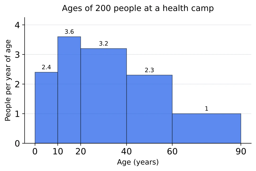
The histogram shows the ages of 200 people at a health camp. The height of each bar is the number of people per year of age in that class.
| Age (years) | 0-10 | 10-20 | 20-40 | 40-60 | 60-90 |
|---|---|---|---|---|---|
| Class width | 10 | 10 | 20 | 20 | 30 |
| Frequency density | 2.4 | 3.6 | 3.2 | 2.3 | 1 |
| Frequency | 24 | 36 | 64 | 46 | 30 |
- The number of people aged 40 to 60 is . Reading the height, 2.3, as the number of people is the first mistake to avoid.
- The tallest bar is 10-20, but the class with the most people is 20-40 (64 against 36). Its bar is lower because its people are spread over twice as many years.
- In such a histogram it is the area of a bar, width times height, that shows its frequency.
Adjusted frequency. The same shape can be drawn another way. Take the narrowest width, 10, as the standard and scale each frequency to it: adjusted frequency . For 20-40 that is , and for 60-90 it is . The heights become 24, 36, 32, 23 and 10, which are the densities multiplied by 10. To read a frequency back, undo the scaling: a bar of height 32 over the class 20-40 stands for people.
Check the vertical axis before reading such a chart. If it says frequency density or 'per unit', multiply by the width; if it says frequency and the classes are unequal, the chart has been drawn with plain frequencies and the heights can be read as they are.
Solved Examples
Question 1
The line graph shows the number of two-wheelers (in hundreds) sold by a dealer from 2017 to 2023.
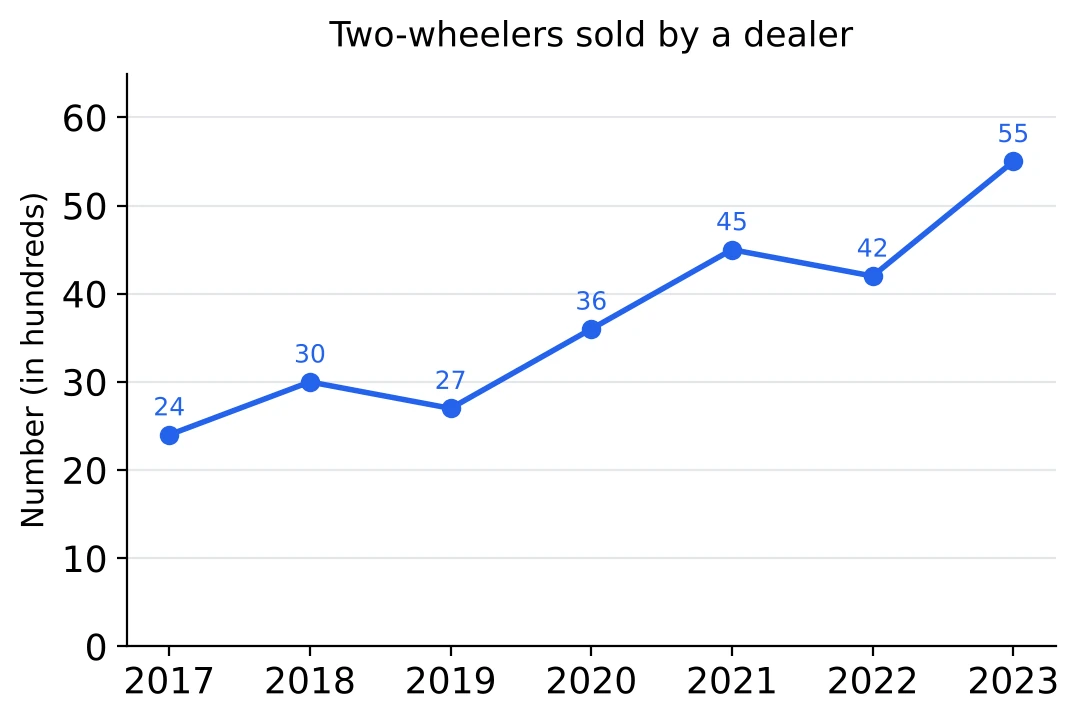
In which year was the increase in sales over the previous year the greatest? (a) 2020 (b) 2023 (c) 2021 (d) 2018
Answer. I go along the line and write the change for each year: 2018 , 2019 , 2020 , 2021 , 2022 , 2023 . The biggest rise is 13 hundred, in (b) 2023, which is also the steepest rising segment on the graph. 2020 had the biggest rise in percentage terms, but the question asks about the number.
Question 2
What was the percentage increase in sales from 2019 to 2020? (a) 25% (b) 9% (c) 50% (d)
Answer. Sales went from 27 hundred to 36 hundred, a rise of 9 hundred. I divide by the earlier year: . So the answer is (d) . The hundreds cancel, so I did not need to change the units.
Question 3
What was the average number of two-wheelers sold per year over the seven years? (a) 3,700 (b) 370 (c) 3,600 (d) 3,950
Answer. Total: hundred. Over 7 years the average is hundred, that is 3,700 two-wheelers a year. The answer is (a) 3,700. The scale is in hundreds, so 37 has to be turned into 3,700; 370 drops a zero.
Question 4
The line graph shows the income and the expenditure of a company (in ₹ crore) from 2019 to 2024.
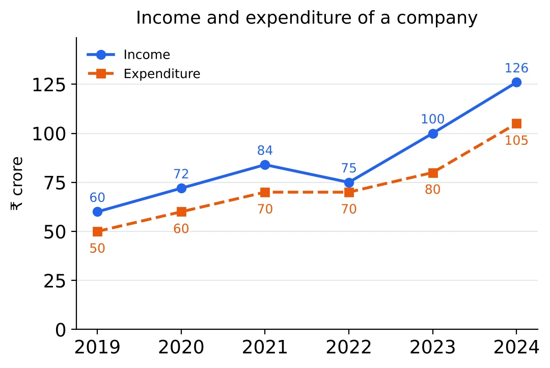
In which year did the company make the largest profit (income minus expenditure)? (a) 2023 (b) 2021 (c) 2024 (d) 2022
Answer. I subtract the lower line from the upper one in every year: 10, 12, 14, 5, 20 and 21 crore from 2019 to 2024. The largest gap is 21 crore, in (c) 2024. 2023 comes close with 20, so I could not have judged this by eye.
Question 5
In which year was the percentage profit the highest? (a) 2023 (b) 2024 (c) 2019 (d) 2021
Answer. Percentage profit is profit divided by expenditure. 2019: , 2020: , 2021: , 2022: , 2023: , 2024: . The highest is 25%, in (a) 2023. The year with the biggest profit in rupees, 2024, earned it on a much bigger expenditure.
Question 6
What was the average expenditure of the company per year over the six years? (a) ₹ 87 crore (b) ₹ 70 crore (c) ₹ 77.5 crore (d) ₹ 72.5 crore
Answer. I add the expenditure points: . Six years, so the average is . The answer is (d) ₹ 72.5 crore. The divisor is the number of points, 6; the five gaps between the years play no part.
Question 7
The line graph shows the percentage profit of two companies P and Q from 2020 to 2024, where .
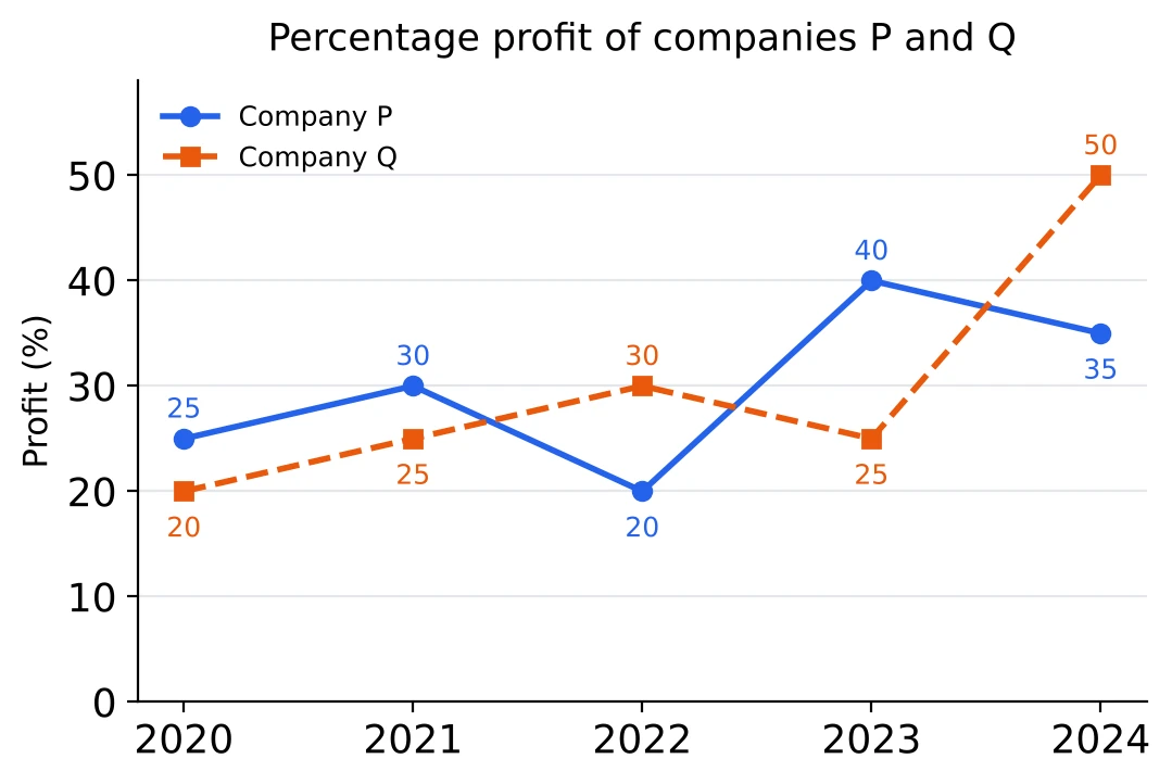
The expenditure of P in 2022 was ₹ 45 crore. What was its income in 2022? (a) ₹ 56.25 crore (b) ₹ 54 crore (c) ₹ 9 crore (d) ₹ 63 crore
Answer. P's profit in 2022 was 20%, so income is expenditure plus 20% of it: . The income was (b) ₹ 54 crore. The 9 crore is only the profit.
Question 8
In 2021 the incomes of P and Q were equal. What was the ratio of the expenditure of P to that of Q in 2021? (a) 26 : 25 (b) 6 : 5 (c) 25 : 26 (d) 5 : 6
Answer. In 2021 P made 30% and Q made 25%. With equal incomes, , so . That is (c) 25 : 26. It makes sense that P, with the higher profit percentage, spent less for the same income.
Question 9
Q's income in 2024 was ₹ 90 crore. What was its expenditure in 2024? (a) ₹ 60 crore (b) ₹ 45 crore (c) ₹ 135 crore (d) ₹ 72 crore
Answer. Q made 50% profit in 2024, so income expenditure. Expenditure , so it was (a) ₹ 60 crore. I divide by 1.5 rather than take half of 90, because the 50% is counted on the expenditure.
Question 10
The histogram shows the weights (in kg) of 120 students of a school.
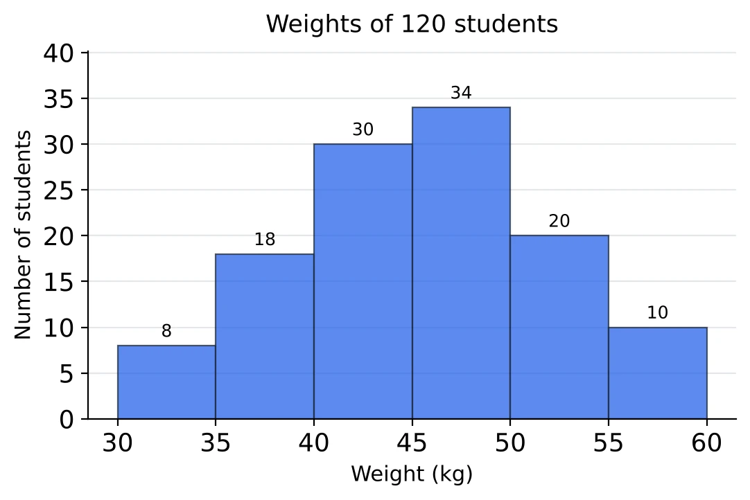
How many students weigh 45 kg or more? (a) 94 (b) 56 (c) 34 (d) 64
Answer. 45 kg or more starts with the bar that begins at 45. I add that bar and the ones after it: . So the answer is (d) 64. Starting one bar early, at 40, would give 94.
Question 11
What percentage of the students weigh less than 40 kg? (a) 15% (b) (c) 26% (d)
Answer. Less than 40 kg means the first two bars: students. As a percentage, . The answer is (b) .
Question 12
What is the ratio of the number of students in the class with the highest frequency to the number in the class 35-40? (a) 5 : 3 (b) 9 : 17 (c) 17 : 9 (d) 17 : 10
Answer. The tallest bar is 45-50, with 34 students. The class 35-40 has 18. So the ratio is , which is (c) 17 : 9.
Question 13
The table shows how many customers visited a shop each day over 40 days.
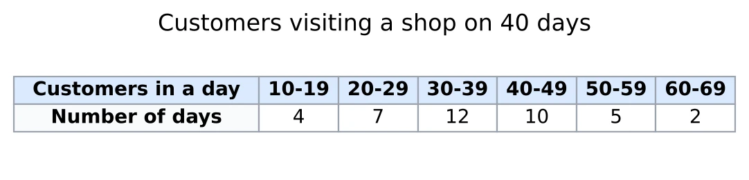
A histogram is drawn from this table. Between which values on the horizontal axis does the bar for the class 30-39 stand? (a) 29.5 and 39.5 (b) 30 and 39 (c) 30 and 40 (d) 29 and 39
Answer. The classes have gaps: 19 is followed by 20, 29 by 30, and so on. The gap is 1, so I take 0.5 away from each lower limit and add 0.5 to each upper limit. The class 30-39 becomes 29.5-39.5, so the answer is (a) 29.5 and 39.5.
Question 14
What is the width of each bar of this histogram? (a) 9 (b) 9.5 (c) 5 (d) 10
Answer. After the change, each class runs from one boundary to the next, for example 29.5 to 39.5, which is . So the width is (d) 10. The 9 comes from subtracting the printed limits, , which leaves out the half-units at both ends.
Question 15
On how many days did at least 40 customers visit the shop? (a) 29 (b) 17 (c) 23 (d) 15
Answer. At least 40 customers means the classes 40-49, 50-59 and 60-69: days. The answer is (b) 17.
Question 16
The frequency polygon shows the distances (in km) run by 75 taxis of a city on one day. The classes are 60-70, 70-80 and so on.
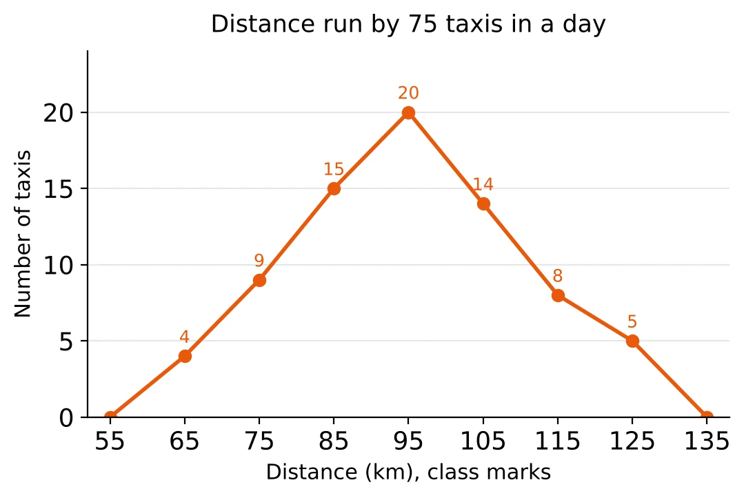
How many taxis ran at least 90 km but less than 110 km? (a) 35 (b) 22 (c) 34 (d) 20
Answer. The classes 90-100 and 100-110 have the class marks 95 and 105. The polygon is at 20 above 95 and at 14 above 105, so taxis. That is (c) 34. The trap is (a) 35: the points above 85 and 95 add up to that, but they stand for the classes 80-90 and 90-100.
Question 17
Which class contains the largest number of taxis? (a) 90-100 (b) 95-105 (c) 85-95 (d) 80-90
Answer. The highest point of the polygon is 20, at the mark 95. The classes are 10 km wide, so the mark 95 stands for 5 km either side of it: 90 to 100. The answer is (a) 90-100.
Question 18
What percentage of the taxis ran 100 km or more? (a) 27% (b) 64% (c) (d) 36%
Answer. 100 km or more means the classes with marks 105, 115 and 125: taxis. Then , which is (d) 36%. 27 is the number of taxis, not the percentage.
Question 19
The frequency polygons show the scores (out of 60) of the 40 students of Batch 1 and the 40 students of Batch 2 of a coaching centre in a test. The classes are 10-20, 20-30, 30-40, 40-50 and 50-60.
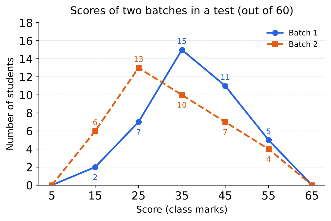
How many more students of Batch 1 than of Batch 2 scored 40 or more? (a) 4 (b) 5 (c) 16 (d) 6
Answer. 40 or more means the classes 40-50 and 50-60, with marks 45 and 55. Batch 1: . Batch 2: . The difference is , so the answer is (b) 5.
Question 20
In which class is the difference between the numbers of students of the two batches the largest? (a) 30-40 (b) 10-20 (c) 20-30 (d) 40-50
Answer. I find the gap between the two polygons at each class mark: at 15, ; at 25, ; at 35, ; at 45, ; at 55, . The largest gap is 6, at the mark 25, which is the class (c) 20-30.
Question 21
[Tier 2] The histogram shows the electricity used in a month by 300 households. The classes are of unequal width, and the height of each bar is the number of households per 10 units in that class.
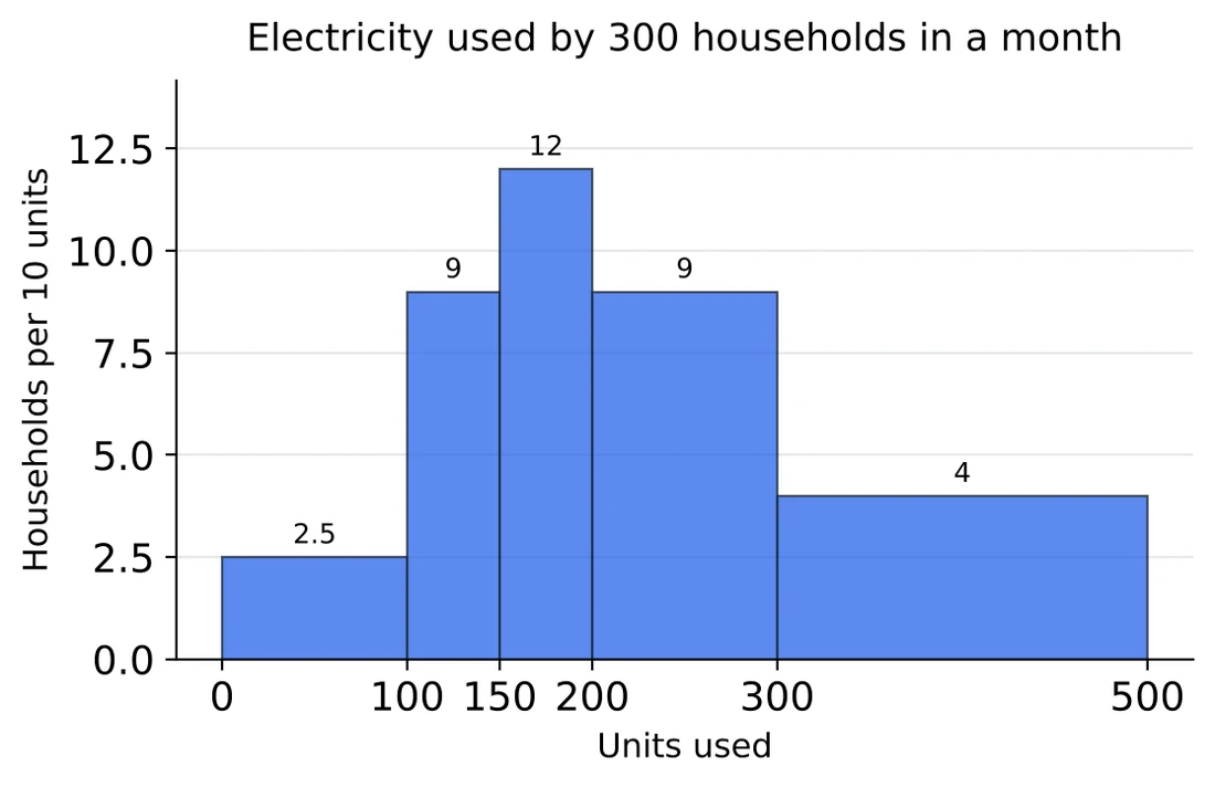
How many households used at least 200 but less than 300 units? (a) 90 (b) 9 (c) 45 (d) 180
Answer. The bar for 200-300 has height 9, which means 9 households for every 10 units. The class is 100 units wide, that is 10 lots of 10 units, so the frequency is . The answer is (a) 90. Reading the height as the number of households would give 9.
Question 22
[Tier 2] How many households used 150 units or more? (a) 25 (b) 150 (c) 275 (d) 230
Answer. I change each bar back into a frequency, the height times the width divided by 10: 150-200 gives , 200-300 gives , and 300-500 gives . In all, households, which is (d) 230.
Question 23
[Tier 2] Which class has the largest number of households? (a) 150-200 (b) 200-300 (c) 300-500 (d) 100-150
Answer. The frequencies are 25, 45, 60, 90 and 80 for the five classes (height times width, as before). The largest is 90, in (b) 200-300. The tallest bar is 150-200, but that class is only 50 units wide, so it holds 60 households.