Integration by Parts

The Product Rule in Reverse

Substitution handles composite functions; integration by parts handles products of functions. It is nothing but the product rule of differentiation, read backwards.

If $u$ and $v$ are differentiable functions of $x$, the product rule says $\frac{d}{dx}(uv) = u\frac{dv}{dx} + v\frac{du}{dx}$. Integrating both sides and rearranging:

$$\int u\,\frac{dv}{dx}\,dx = uv - \int v\,\frac{du}{dx}\,dx$$

Writing $u = f(x)$ (the first function) and $\frac{dv}{dx} = g(x)$ (the second function), this becomes the working formula:

$$\int f(x)\,g(x)\,dx = f(x)\int g(x)\,dx \;-\; \int\left[f'(x)\int g(x)\,dx\right]dx$$

In words (NCERT's statement): the integral of the product of two functions = (first function) × (integral of the second function) − integral of [(derivative of the first function) × (integral of the second function)].

Choosing the first function — why it matters

Try $\int x\cos x\,dx$ both ways. With $f = x$, $g = \cos x$: the new integral is $\int \sin x\,dx$ — easier, and we finish with $x\sin x + \cos x + C$. With $f = \cos x$, $g = x$: the new integral is $\int \frac{x^2}{2}\sin x\,dx$ — harder than what we started with, because the power of $x$ went up. The proper choice of first function decides whether by parts helps or hurts.

NCERT's rule of thumb: take the power of $x$ (or polynomial) as the first function — except when the other function is an inverse trigonometric or logarithmic function, in which case that becomes the first function (its derivative is algebraic and simpler, and it often has no elementary integral to serve as second function).

The ILATE memory aid: pick as first function whichever comes earlier in the list — Inverse trig, Logarithmic, Algebraic, Trigonometric, Exponential. It encodes exactly NCERT's advice: $\log x$ and $\tan^{-1}x$ beat $x^2$, and $x^2$ beats $\sin x$ and $e^x$.

Key Point: By parts trades one integral for another. The trade is good only if $f'(x)\int g(x)\,dx$ is easier to integrate than $f(x)g(x)$ — choose the first function so that differentiating it simplifies it.

Three remarks from NCERT

1. By parts is not universal. It applies to products, but not to every product: $\int \sqrt{x}\,\sin x\,dx$ cannot be done by parts (no choice works — there is no elementary answer at all).
2. No constant with the second function. While computing $\int g(x)\,dx$ inside the formula, do not add a constant: if you write $\sin x + k$ instead of $\sin x$, the $k$-terms cancel in the final answer. The constant $C$ appears once, at the very end.
3. Functions without visible products. $\int \log x\,dx$ and $\int \tan^{-1}x\,dx$ have no product — until you write them as $\log x \cdot 1$ and $\tan^{-1}x \cdot 1$, take the constant function $1$ as the second function, and integrate by parts. This trick is examined constantly.

[JEE Tip] In JEE Main, by-parts questions are rarely a single application: expect two rounds (as in $\int x^2 e^x dx$), a loop back to the original integral (as in $\int e^x\sin x\,dx$), or the disguised $e^x[f + f']$ pattern of the next block. Learn to recognise which of the three scripts is running before you start writing.

Two Special Patterns Built on By Parts

Pattern 1: $\int e^x[f(x) + f'(x)]\,dx = e^x f(x) + C$

Split the integral: $\int e^x f(x)\,dx + \int e^x f'(x)\,dx$. Integrate the first piece by parts (with $f$ as first function): it equals $e^x f(x) - \int e^x f'(x)\,dx$. The two $\int e^x f'(x)\,dx$ terms cancel, leaving

$$\int e^x\left[f(x) + f'(x)\right]dx = e^x f(x) + C$$

The skill is recognition: given $\int e^x(\text{something})\,dx$, ask whether the bracket splits as some function plus its own derivative. For example, in $\int e^x\left(\tan^{-1}x + \frac{1}{1+x^2}\right)dx$, the bracket is $f + f'$ with $f = \tan^{-1}x$ — answer $e^x\tan^{-1}x + C$, no working needed.

Key Point: Whenever $e^x$ multiplies a sum of two terms, test whether one term is the derivative of the other. If yes, the answer is $e^x \times (\text{the original term})+ C$ — the one whose derivative also appears.

Pattern 2: the three square-root integrals (NCERT 7.6.2)

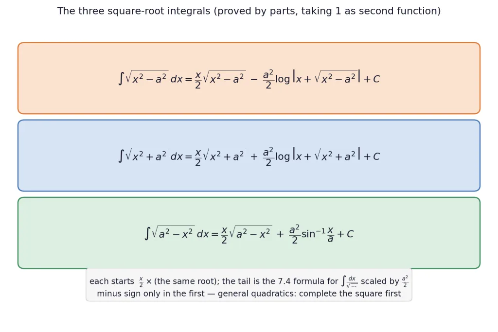
Taking $1$ as the second function and integrating by parts (the integral loops back to itself, just like $\int e^x \sin x\,dx$), NCERT derives three more standard results:

1. $\displaystyle\int \sqrt{x^2 - a^2}\,dx = \frac{x}{2}\sqrt{x^2 - a^2} - \frac{a^2}{2}\log\left|x + \sqrt{x^2 - a^2}\right| + C$
2. $\displaystyle\int \sqrt{x^2 + a^2}\,dx = \frac{x}{2}\sqrt{x^2 + a^2} + \frac{a^2}{2}\log\left|x + \sqrt{x^2 + a^2}\right| + C$
3. $\displaystyle\int \sqrt{a^2 - x^2}\,dx = \frac{x}{2}\sqrt{a^2 - x^2} + \frac{a^2}{2}\sin^{-1}\frac{x}{a} + C$

Memory scheme: every answer starts $\frac{x}{2}\sqrt{\cdots}$ (half of $x$ times the same root). The tail copies the Section 7.4 formula for the reciprocal of that root, scaled by $\frac{a^2}{2}$ — a log for $x^2 \pm a^2$, a $\sin^{-1}$ for $a^2 - x^2$ — with a minus sign only in the first formula.

General quadratics. For $\int\sqrt{ax^2 + bx + c}\,dx$, complete the square, substitute the shifted variable, and apply whichever of the three fits — exactly the Section 7.4 workflow, now with the root outside the denominator. (Alternatively the three can be derived by the trigonometric substitutions $x = a\sec\theta$, $x = a\tan\theta$, $x = a\sin\theta$ respectively.)

[JEE Tip] These three formulas are in the JEE Main syllabus and appear directly — usually after a completing-the-square step. Quote them; deriving by parts under exam pressure wastes three minutes.

Solved Examples

Example 1: The model case

Find $\displaystyle\int x\cos x\,dx$.

Solution:

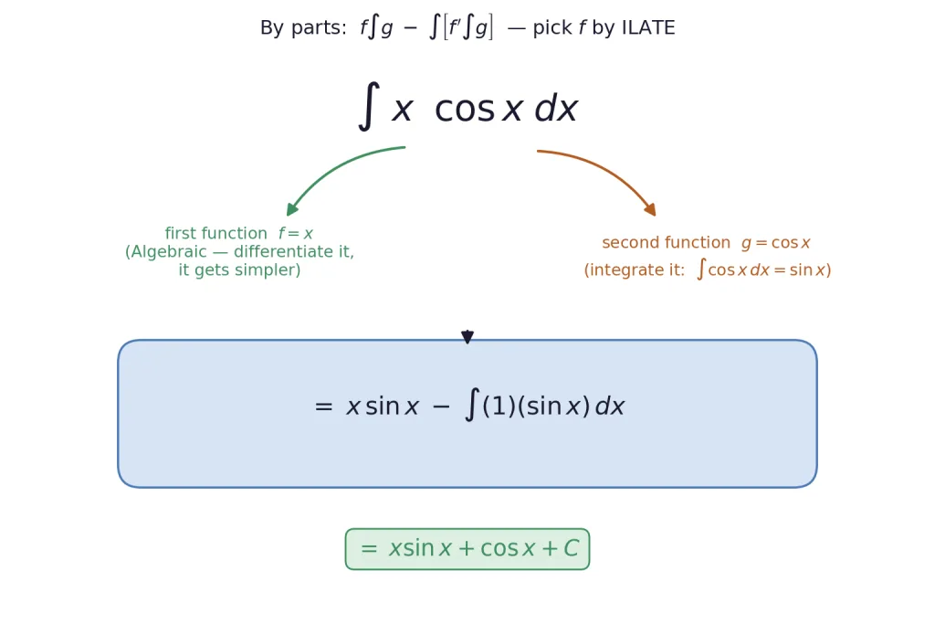
1. Choose: ILATE — Algebraic $x$ before Trigonometric $\cos x$, so $f = x$, $g = \cos x$.
2. Apply the formula: $\int x\cos x\,dx = x\sin x - \int (1)(\sin x)\,dx$.
3. Finish: $= x\sin x + \cos x + C$.

Final Answer: $x\sin x + \cos x + C$.

Takeaway: Check by differentiating: $\frac{d}{dx}(x\sin x + \cos x) = \sin x + x\cos x - \sin x = x\cos x$. ✓

Example 2: The constant-function trick

Find $\displaystyle\int \log x\,dx$.

Solution:

1. Create a product: write $\log x = (\log x)\cdot 1$; take $f = \log x$ (Logarithmic), $g = 1$.
2. Apply: $\int \log x\,dx = (\log x)(x) - \int \frac{1}{x}\cdot x\,dx$.
3. Finish: $= x\log x - \int 1\,dx = x\log x - x + C$.

Final Answer: $x\log x - x + C$.

Example 3: Polynomial times exponential

Find $\displaystyle\int x e^x\,dx$.

Solution:

1. Choose: $f = x$ (Algebraic before Exponential), $g = e^x$.
2. Apply: $\int x e^x dx = x e^x - \int 1\cdot e^x dx = x e^x - e^x + C$.

Final Answer: $(x - 1)e^x + C$.

Example 4: By parts twice

Find $\displaystyle\int x^2 e^x\,dx$.

Solution:

1. Round 1: $f = x^2$, $g = e^x$: $\int x^2 e^x dx = x^2 e^x - 2\int x e^x dx$.
2. Round 2: by Example 3, $\int x e^x dx = (x-1)e^x$.
3. Combine: $x^2 e^x - 2(x - 1)e^x + C = (x^2 - 2x + 2)e^x + C$.

Final Answer: $(x^2 - 2x + 2)e^x + C$.

Takeaway: Each round of by parts drops the power of $x$ by one. A polynomial of degree $n$ times $e^x$ needs $n$ rounds — and the signs alternate.

Example 5: Inverse trig as first function

Find $\displaystyle\int x\tan^{-1}x\,dx$.

Solution:

1. Choose: ILATE — Inverse $\tan^{-1}x$ before Algebraic $x$, so $f = \tan^{-1}x$, $g = x$.
2. Apply: $\int x\tan^{-1}x\,dx = \tan^{-1}x\cdot\frac{x^2}{2} - \frac{1}{2}\int \frac{x^2}{1 + x^2}\,dx$.
3. Simplify the remainder: $\frac{x^2}{1+x^2} = 1 - \frac{1}{1+x^2}$, so $\int \frac{x^2}{1+x^2}dx = x - \tan^{-1}x$.
4. Combine: $\frac{x^2}{2}\tan^{-1}x - \frac{x}{2} + \frac{1}{2}\tan^{-1}x + C$.

Final Answer: $\frac{1}{2}(x^2 + 1)\tan^{-1}x - \frac{x}{2} + C$.

Takeaway: The add-and-subtract move $\frac{x^2}{1+x^2} = 1 - \frac{1}{1+x^2}$ is the standard finisher whenever by parts leaves a proper-degree rational function.

Example 6: A hybrid with substitution

Find $\displaystyle\int \frac{x\sin^{-1}x}{\sqrt{1 - x^2}}\,dx$.

Solution:

1. Choose: $f = \sin^{-1}x$ (first), $g = \frac{x}{\sqrt{1-x^2}}$ (second).
2. Integrate the second function: put $t = 1 - x^2$, $dt = -2x\,dx$: $\int\frac{x\,dx}{\sqrt{1-x^2}} = -\frac{1}{2}\int\frac{dt}{\sqrt t} = -\sqrt t = -\sqrt{1 - x^2}$.
3. Apply by parts: $\int\frac{x\sin^{-1}x}{\sqrt{1-x^2}}dx = \sin^{-1}x\cdot(-\sqrt{1-x^2}) - \int\frac{1}{\sqrt{1-x^2}}\cdot(-\sqrt{1-x^2})\,dx$.
4. Finish: $= -\sqrt{1-x^2}\,\sin^{-1}x + \int 1\,dx = x - \sqrt{1-x^2}\,\sin^{-1}x + C$.

Final Answer: $x - \sqrt{1 - x^2}\,\sin^{-1}x + C$.

Example 7: The loop-back integral

Find $\displaystyle\int e^x\sin x\,dx$.

Solution:

1. Round 1 ($f = e^x$, $g = \sin x$): $I = e^x(-\cos x) + \int e^x\cos x\,dx = -e^x\cos x + I_1$.
2. Round 2 on $I_1$ ($f = e^x$, $g = \cos x$): $I_1 = e^x\sin x - \int e^x\sin x\,dx = e^x\sin x - I$.
3. The loop: $I = -e^x\cos x + e^x\sin x - I$, so $2I = e^x(\sin x - \cos x)$.

Final Answer: $\displaystyle\int e^x \sin x\,dx = \frac{e^x}{2}(\sin x - \cos x) + C$.

Takeaway: When the original integral reappears on the right, don't panic — move it to the left and solve algebraically for $I$. Keep the same choice-type of first function in both rounds, or the two rounds undo each other.

Example 8: Spotting $e^x[f + f']$

Find $\displaystyle\int e^x\left(\tan^{-1}x + \frac{1}{1 + x^2}\right)dx$.

Solution:

1. Test the bracket: with $f = \tan^{-1}x$, $f' = \frac{1}{1+x^2}$ — the bracket is exactly $f + f'$.
2. Quote the pattern: $\int e^x[f + f']\,dx = e^x f(x) + C$.

Final Answer: $e^x\tan^{-1}x + C$.

Example 9: Hidden $f + f'$

Find $\displaystyle\int \frac{(x^2 + 1)e^x}{(x + 1)^2}\,dx$.

Solution:

1. Rewrite the numerator: $x^2 + 1 = (x^2 - 1) + 2$, so the integrand is $e^x\left[\frac{x^2-1}{(x+1)^2} + \frac{2}{(x+1)^2}\right] = e^x\left[\frac{x-1}{x+1} + \frac{2}{(x+1)^2}\right]$.
2. Test: with $f = \frac{x-1}{x+1}$, the quotient rule gives $f' = \frac{(x+1) - (x-1)}{(x+1)^2} = \frac{2}{(x+1)^2}$ — again $f + f'$.

Final Answer: $\dfrac{x - 1}{x + 1}\,e^x + C$.

Takeaway: The $f + f'$ pattern is often disguised by algebra. When $e^x$ multiplies a rational function, split it into two pieces and check whether one is the derivative of the other.

Example 10: A trig disguise

Find $\displaystyle\int e^x\left(\frac{1 + \sin x}{1 + \cos x}\right)dx$.

Solution:

1. Half-angle everything: $1 + \cos x = 2\cos^2\frac{x}{2}$ and $1 + \sin x = \left(\sin\frac{x}{2} + \cos\frac{x}{2}\right)^2$… a cleaner split: $\frac{1+\sin x}{1+\cos x} = \frac{1}{2}\sec^2\frac{x}{2} + \tan\frac{x}{2}$ (using $\sin x = 2\sin\frac{x}{2}\cos\frac{x}{2}$).
2. Test: with $f = \tan\frac{x}{2}$, $f' = \frac{1}{2}\sec^2\frac{x}{2}$ — the bracket is $f + f'$.

Final Answer: $e^x\tan\dfrac{x}{2} + C$.

Example 11: Completing the square under the root

Find $\displaystyle\int \sqrt{x^2 + 2x + 5}\,dx$.

Solution:

1. Complete the square: $x^2 + 2x + 5 = (x+1)^2 + 4$.
2. Shift: put $y = x + 1$, $dy = dx$: the integral is $\int\sqrt{y^2 + 2^2}\,dy$ — root formula (2).
3. Apply: $\frac{y}{2}\sqrt{y^2 + 4} + \frac{4}{2}\log\left|y + \sqrt{y^2 + 4}\right| + C$.
4. Return to $x$: substitute $y = x + 1$ back.

Final Answer: $\dfrac{x+1}{2}\sqrt{x^2 + 2x + 5} + 2\log\left|x + 1 + \sqrt{x^2 + 2x + 5}\right| + C$.

Example 12: The $\sin^{-1}$ case

Find $\displaystyle\int \sqrt{3 - 2x - x^2}\,dx$.

Solution:

1. Complete the square: $3 - 2x - x^2 = 4 - (x+1)^2$.
2. Shift: $y = x + 1$: the integral is $\int\sqrt{2^2 - y^2}\,dy$ — root formula (3).
3. Apply: $\frac{y}{2}\sqrt{4 - y^2} + \frac{4}{2}\sin^{-1}\frac{y}{2} + C$.
4. Return: $y = x+1$.

Final Answer: $\dfrac{x+1}{2}\sqrt{3 - 2x - x^2} + 2\sin^{-1}\left(\dfrac{x+1}{2}\right) + C$.

Takeaway: Same decision rule as Section 7.4: minus in front of $x^2$ under the root → the $\sin^{-1}$ formula; plus → a log formula. The completed square hands you the shift and the value of $a$.

Example 13: Scaling first

Find $\displaystyle\int \sqrt{1 - 4x^2}\,dx$.

Solution:

1. Factor out the coefficient: $\sqrt{1 - 4x^2} = 2\sqrt{\frac{1}{4} - x^2}$, so the integral is $2\int\sqrt{\left(\frac{1}{2}\right)^2 - x^2}\,dx$.
2. Apply formula (3) with $a = \frac{1}{2}$: $2\left[\frac{x}{2}\sqrt{\tfrac{1}{4} - x^2} + \frac{1}{8}\sin^{-1}(2x)\right] + C$.
3. Tidy: $x\sqrt{\tfrac14 - x^2} = \frac{x}{2}\sqrt{1 - 4x^2}$.

Final Answer: $\dfrac{x}{2}\sqrt{1 - 4x^2} + \dfrac{1}{4}\sin^{-1}(2x) + C$.

Example 14: A root with real zeros

Find $\displaystyle\int \sqrt{x^2 + 4x - 5}\,dx$.

Solution:

1. Complete the square: $x^2 + 4x - 5 = (x+2)^2 - 9$.
2. Shift: $y = x + 2$: integral becomes $\int\sqrt{y^2 - 3^2}\,dy$ — root formula (1), the one with the minus sign.
3. Apply: $\frac{y}{2}\sqrt{y^2 - 9} - \frac{9}{2}\log\left|y + \sqrt{y^2 - 9}\right| + C$.
4. Return: $y = x + 2$.

Final Answer: $\dfrac{x+2}{2}\sqrt{x^2 + 4x - 5} - \dfrac{9}{2}\log\left|x + 2 + \sqrt{x^2 + 4x - 5}\right| + C$.

Takeaway: Only the $\sqrt{x^2 - a^2}$ formula carries a minus sign before the log term — the sign of $a^2$ in the completed square tells you which formula (and which sign) you need.