JEE Corner — Errors in Measurement and Advanced Dimensional Analysis

Every Measurement Is Wrong. The Only Question Is How Wrong.

Welcome to the part of Chapter 1 that your NCERT textbook no longer prints — and that JEE Main and JEE Advanced ask about every single year. The 2023 rationalisation trimmed error analysis out of the Class 11 book, but nobody told the exam. So this section teaches the whole topic from scratch. Assume nothing; we build it up from zero.

Section 3 already gave you the Board-level version: uncertainty in a calculated result, percentage errors adding for a product. Here we go all the way — where errors come from, how to classify them, how to average them honestly, how to derive the combination rules rather than just quote them, and how to read a vernier calliper and a screw gauge.

The starting point

Key Point (Definition): The error in a measurement is the difference between the measured value and the true value of the quantity.

Every measurement has one. Not because you were sloppy, but because instruments have finite resolution, conditions drift and human beings are involved. So the honest scientific question is never "is my answer right?" — it is "how far off could it be?"

Accuracy and precision are not the same word

Students use these two interchangeably in ordinary English. Physics does not, and examiners know it.

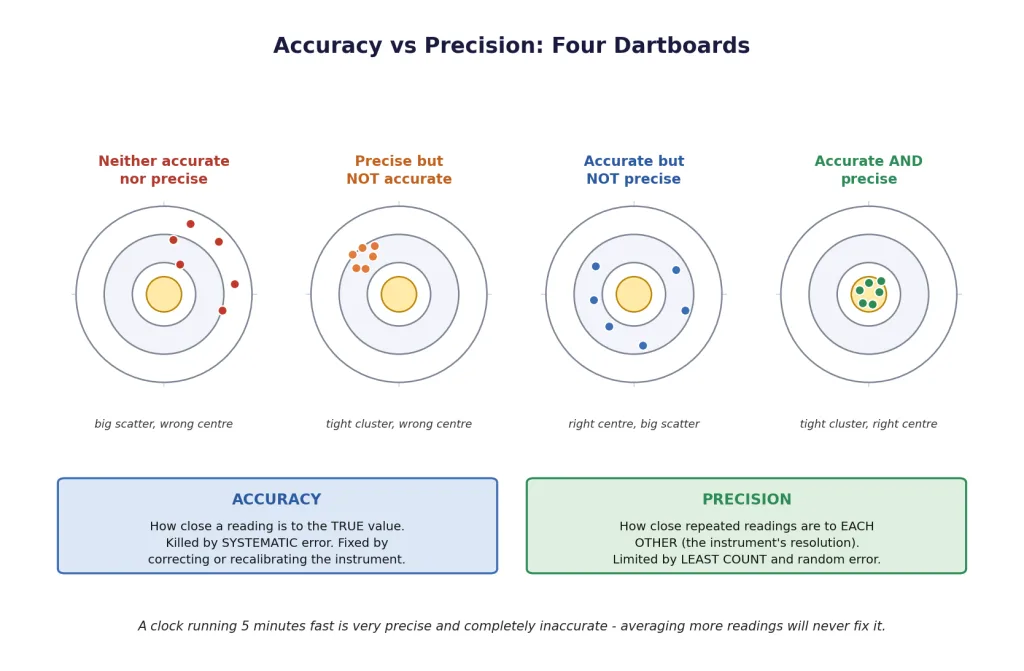
Key Point (Definition): Accuracy is a measure of how close a measured value is to the true value of the quantity.

Precision tells you to what resolution the quantity is measured — how finely, and how consistently, repeated readings agree with one another.

The example that makes it click

Suppose the true length of a rod is 3.678 cm. Two students measure it:

Student	Instrument	Readings	Verdict
A	metre scale	3.5, 3.6, 3.5, 3.6 cm	accurate (close to 3.678) but not precise (only 2 figures)
B	faulty vernier	3.421, 3.422, 3.421, 3.423 cm	precise (agree to 0.001 cm) but not accurate

Student B's instrument is better and B's answer is worse. Read that again — it is the entire point.

Key Point: A measurement can be precise but inaccurate. Tight, repeatable readings that all sit around the wrong value mean the instrument is finely divided and wrongly calibrated. No amount of repeating will reveal it.

[Exam Tip] The classic exam framing: a clock that runs 5 minutes fast is extremely precise — it will give you the same wrong answer to the second, all day. Precision is about agreement, accuracy about truth. And here is the consequence that matters for the next block: averaging many readings improves precision, never accuracy.

Where the two come from

• Poor accuracy comes from systematic error, which pushes every reading the same way.
• Poor precision comes from random error and from the least count of the instrument.

Those are the next two things we have to define properly.

Systematic Errors and Random Errors

All errors in measurement sort into two families, and they are treated completely differently.

Key Point (Definition): Systematic errors are those errors that tend to be in one direction only — either always positive or always negative. Because they have a definite sign and cause, they can in principle be identified and corrected for.

The three sources of systematic error

1. Instrumental errors. The instrument itself is imperfect.

• A vernier calliper whose jaws do not read zero when closed (zero error — a whole block below).
• A thermometer graduated in $0.2\ ^\circ$C steps but calibrated so it reads $0.5\ ^\circ$C high.
• A metre scale worn away at the zero end, so every length comes out short.
• An ammeter whose needle rests slightly off zero.

2. Imperfection in experimental technique or procedure. The method has a built-in bias.

• Measuring body temperature with a thermometer under the armpit: the reading is always lower than the true body temperature.
• Ignoring the buoyancy of air while weighing — every mass reads slightly low.
• Ignoring heat lost to the surroundings in a calorimetry experiment.

3. Personal errors. The observer contributes a consistent bias.

• Parallax: reading a scale from an angle instead of straight on, so you always read high (or always low).
• Carelessness in setting the apparatus, or in taking the observation without proper precautions.
• A habit of pressing the stopwatch a fraction of a second late on every single trial.

Key Point: Systematic errors are minimised by using better instruments, improving the experimental technique, removing personal bias, and applying a correction for the known error. They are not reduced by taking more readings — repeating a biased measurement just gives you the same bias, more confidently.

Random errors

Key Point (Definition): Random errors are those errors which occur irregularly and are random with respect to sign and size. They arise from unpredictable fluctuations in experimental conditions (temperature, voltage supply, vibration) and from personal fluctuations by the observer.

The stopwatch example again: sometimes you press it 0.1 s early, sometimes 0.15 s late, with no pattern. Because the deviations scatter on both sides of the true value, they partly cancel when you average.

Key Point: Random errors are minimised by taking a large number of observations and using their arithmetic mean. This is the whole reason lab manuals ask for five readings instead of one.

	Systematic error	Random error
Sign	always the same	varies, both signs
Cause	traceable and definite	unpredictable fluctuations
Effect on the result	destroys accuracy	destroys precision
How to reduce	correct or recalibrate; better technique	repeat and average
Does averaging help?	No	Yes

Least count error

Key Point (Definition): The smallest value that can be measured by a measuring instrument is called its least count. The least count error is the error associated with the resolution of the instrument.

A metre scale with millimetre divisions has a least count of 1 mm, so a length read on it carries an uncertainty of $\pm 1$ mm — you simply cannot do better with that scale. A vernier calliper has a least count of 0.01 cm, a screw gauge 0.001 cm.

Least count error is a slightly odd creature: it belongs with the random errors, but it is bounded — it can never exceed the least count itself. It sets a hard floor on how precise any single reading can be.

Key Point: Least count error is reduced by using instruments of higher precision and improving the experimental technique — never by repeating readings, because every reading hits the same floor.

[Important] When a problem gives you an instrument but no explicit uncertainty, the intended $\Delta a$ is the least count. "A length of 2.50 cm measured with a vernier calliper of least count 0.01 cm" means $\Delta a = 0.01$ cm, a relative error of $0.01/2.50 = 0.004$, or 0.4%.

Absolute Error, Mean Absolute Error, Relative Error, Percentage Error

Now the bookkeeping. You have taken $n$ readings of a quantity $a$ and they disagree. What single number do you report, and with what $\pm$?

Step 1: the true value is the mean

The true value is unknowable. But the arithmetic mean of many readings is our best estimate of it, because random errors cancel on averaging.

$$a_{mean} = \frac{a_1 + a_2 + \cdots + a_n}{n} = \frac{1}{n}\sum_{i=1}^{n} a_i$$

Step 2: absolute error of each reading

Key Point (Definition): The absolute error of a measurement is the magnitude of the difference between the individual measured value and the true value (in practice, the mean) of the quantity.

$$\Delta a_i = a_{mean} - a_i \qquad \text{and we always take its magnitude } |\Delta a_i|$$

Absolute error carries the same unit as the quantity itself. If $a$ is in seconds, $\Delta a$ is in seconds.

Step 3: mean absolute error

Key Point (Definition): The arithmetic mean of all the absolute errors, taken as positive quantities, is called the mean absolute error:

$$\Delta a_{mean} = \frac{|\Delta a_1| + |\Delta a_2| + \cdots + |\Delta a_n|}{n} = \frac{1}{n}\sum_{i=1}^{n} |\Delta a_i|$$

Take the magnitudes before averaging. If you forget, the deviations cancel and you get zero — which is exactly why the modulus signs are there.

Step 4: report the result

Key Point: The final result is quoted as $$a = a_{mean} \pm \Delta a_{mean}$$ which says that any measurement of $a$ is likely to lie between $a_{mean} - \Delta a_{mean}$ and $a_{mean} + \Delta a_{mean}$.

Relative and percentage error

An absolute error of 1 cm is trivial on a road and catastrophic on a screw thread. So we compare it with the quantity being measured.

Key Point (Definition): The relative error (or fractional error) is the ratio of the mean absolute error to the mean value: $$\text{relative error} = \frac{\Delta a_{mean}}{a_{mean}}$$ Expressed as a percentage, it is called the percentage error $\delta a$: $$\delta a = \frac{\Delta a_{mean}}{a_{mean}} \times 100\%$$

Relative and percentage error are pure numbers — no units. That is precisely what makes them combinable across quantities of different kinds, which the next block exploits.

Quantity	Symbol	Formula	Unit
Mean value	$a_{mean}$	$\frac{1}{n}\sum a_i$	same as $a$
Absolute error of a reading	$\vert\Delta a_i\vert$	$\vert a_{mean} - a_i\vert$	same as $a$
Mean absolute error	$\Delta a_{mean}$	$\frac{1}{n}\sum \vert\Delta a_i\vert$	same as $a$
Relative error	—	$\frac{\Delta a_{mean}}{a_{mean}}$	none
Percentage error	$\delta a$	$\frac{\Delta a_{mean}}{a_{mean}} \times 100$	none (%)

[Exam Tip] Section 3 showed you why the same absolute error can mean wildly different relative errors: $\pm 0.01$ g on a 1.02 g sample is 1%, but on a 9.89 g sample it is only 0.1%. Same balance, ten times the quality. Whenever an experiment lets you choose, measure the biggest sample and the longest time you can — it shrinks the relative error for free.

Combination of Errors: Deriving All Four Rules

Real quantities are calculated, not measured. Density comes from a mass and a volume; $g$ comes from a length and a time. So how do the input errors flow into the answer?

Section 3 handed you the answer. Here we derive it, because JEE Advanced asks you to apply it in shapes you have never seen.

Rule 1: error of a sum

Let $Z = A + B$, with $A \pm \Delta A$ and $B \pm \Delta B$. Then

$$Z \pm \Delta Z = (A \pm \Delta A) + (B \pm \Delta B) = (A + B) \pm (\Delta A + \Delta B)$$

The maximum possible error happens when both measurements err the same way, so

$$\Delta Z = \Delta A + \Delta B$$

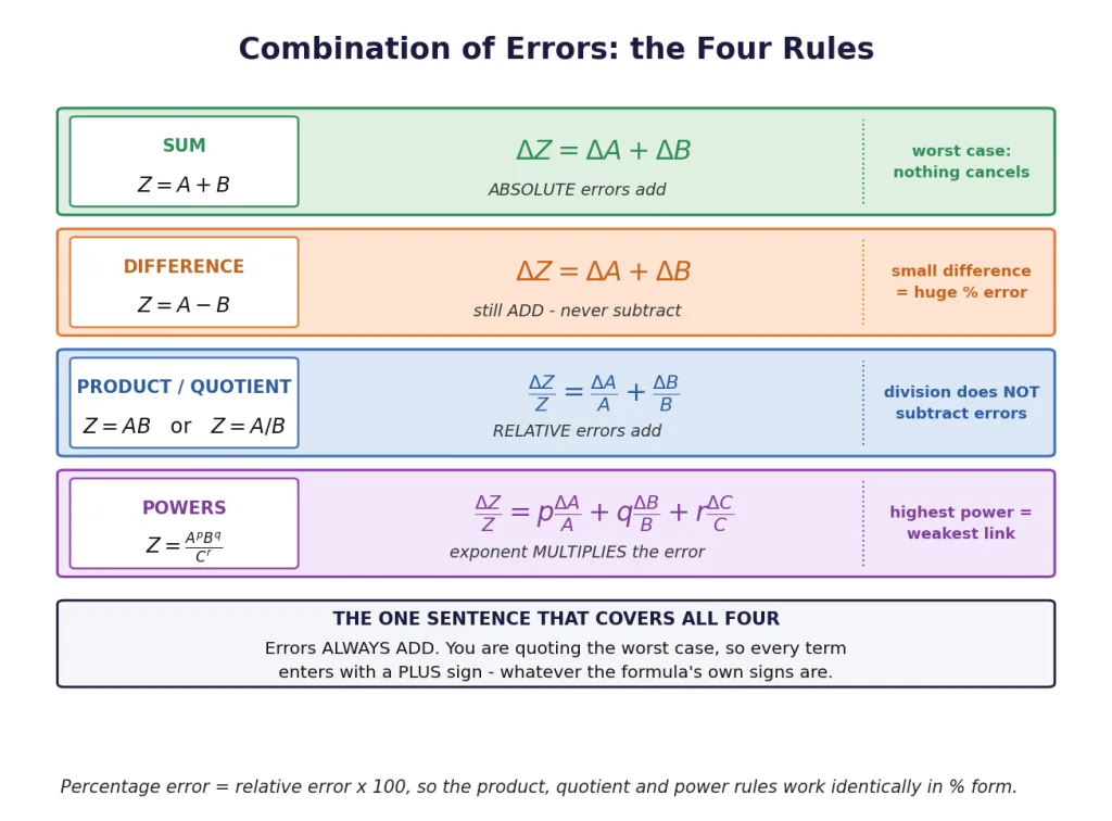
Key Point (Rule 1): When two quantities are added, the absolute error in the final result is the sum of the absolute errors.

Rule 2: error of a difference

Let $Z = A - B$. Now

$$Z \pm \Delta Z = (A \pm \Delta A) - (B \mp \Delta B) = (A - B) \pm (\Delta A + \Delta B)$$

Look at the sign carefully. The worst case for a difference is $A$ too big and $B$ too small — both push $Z$ up. So once again

$$\Delta Z = \Delta A + \Delta B$$

Key Point (Rule 2): When two quantities are subtracted, the absolute errors still ADD. They never subtract.

[Exam Tip] This is where marks disappear. Subtracting two nearly equal numbers keeps the absolute error the same while shrinking the result, so the percentage error explodes. Measuring $25.0 \pm 0.5$ and $20.0 \pm 0.5$ (2% and 2.5% each) gives a difference of $5.0 \pm 1.0$ — a 20% error. Good experimental design avoids taking small differences of large numbers.

Rule 3: error of a product or a quotient

Let $Z = AB$. Then

$$Z \pm \Delta Z = (A \pm \Delta A)(B \pm \Delta B) = AB \pm A\,\Delta B \pm B\,\Delta A + \Delta A\,\Delta B$$

Divide throughout by $Z = AB$:

$$1 \pm \frac{\Delta Z}{Z} = 1 \pm \frac{\Delta B}{B} \pm \frac{\Delta A}{A} + \frac{\Delta A}{A}\cdot\frac{\Delta B}{B}$$

The last term is a product of two small fractions — a second-order quantity. If each relative error is around 1%, that term is around 0.01%, utterly negligible, so we drop it. Taking the worst case again:

$$\frac{\Delta Z}{Z} = \frac{\Delta A}{A} + \frac{\Delta B}{B}$$

For a quotient $Z = A/B$ the same thing happens: expand $(1 + \Delta B/B)^{-1} \approx 1 - \Delta B/B$ by the binomial theorem, and the worst case once more gives a plus.

Key Point (Rule 3): When two quantities are multiplied or divided, the relative error in the result is the sum of the relative errors in the multipliers. Division does not subtract errors.

Rule 4: error in a quantity raised to a power

If $Z = A^2 = A \times A$, Rule 3 applied to the two factors gives $\frac{\Delta Z}{Z} = \frac{\Delta A}{A} + \frac{\Delta A}{A} = 2\frac{\Delta A}{A}$. Repeat the argument $p$ times and the general result follows.

Key Point (Rule 4): If $$Z = \frac{A^p B^q}{C^r}$$ then $$\frac{\Delta Z}{Z} = p\,\frac{\Delta A}{A} + q\,\frac{\Delta B}{B} + r\,\frac{\Delta C}{C}$$ Every exponent enters as a positive multiplier, whether it sat upstairs or downstairs, and whether it is a whole number, a fraction or negative — you use its magnitude.

The two sentences to carry into the exam

Key Point: (1) Errors always add — you are quoting a worst case, so nothing ever cancels. (2) The exponent multiplies the relative error, so the quantity raised to the highest power dominates the error budget.

The classic "which measurement matters most" question

Take $Z = \dfrac{A^2 B^{1/2}}{C^{1/3} D^3}$ with percentage errors $A$: 1%, $B$: 2%, $C$: 3%, $D$: 0.5%. The contributions are

Quantity	Power	Percentage error	Contribution
$A$	2	1%	$2 \times 1 = 2.0$%
$B$	$\frac{1}{2}$	2%	$0.5 \times 2 = 1.0$%
$C$	$\frac{1}{3}$	3%	$\frac{1}{3} \times 3 = 1.0$%
$D$	3	0.5%	$3 \times 0.5 = 1.5$%
			total 5.5%

$C$ has the sloppiest measurement (3%) yet contributes the least. $A$ has one of the tidiest (1%) and contributes the most, because of that exponent 2. Take the most care over the quantity with the largest power, not the largest error.

The Vernier Callipers

Two instruments account for almost every least-count question ever asked. Here is the first.

A metre scale stops at 1 mm. The vernier gets you a factor of ten better with no finer engraving at all — by the elegant trick of making the sliding scale's divisions slightly smaller than the main scale's.

The construction

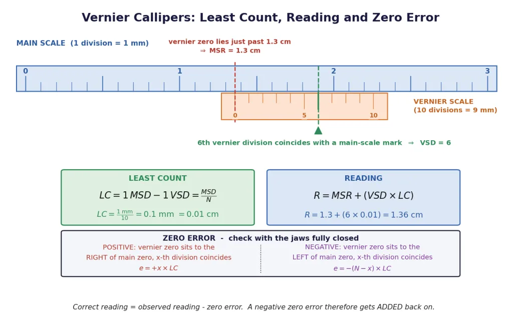
A vernier calliper has a fixed main scale (MS), usually graduated in millimetres, and a sliding vernier scale (VS) carrying $N$ divisions. The scales are cut so that

$$N \text{ vernier divisions} = (N - 1) \text{ main scale divisions}$$

For the common instrument $N = 10$: ten vernier divisions span exactly 9 mm, so one vernier division is 0.9 mm — a whisker smaller than a main division.

Least count

Key Point (Definition): The least count of a vernier calliper is the difference between one main scale division and one vernier scale division: $$LC = 1\ MSD - 1\ VSD$$

Since $1\ VSD = \frac{N-1}{N} MSD$,

$$LC = MSD - \frac{N-1}{N}MSD = \frac{MSD}{N}$$

Key Point (the working formula): $$LC = \frac{\text{value of 1 main scale division}}{\text{number of divisions on the vernier scale}} = \frac{MSD}{N}$$

$MSD$	$N$	Least count
1 mm	10	0.1 mm $= 0.01$ cm
1 mm	20	0.05 mm $= 0.005$ cm
1 mm	50	0.02 mm $= 0.002$ cm
0.5 mm	25	0.02 mm $= 0.002$ cm

Taking a reading

Key Point: $$\text{Reading} = MSR + (n \times LC)$$ where MSR (main scale reading) is the main scale mark just before the vernier zero, and $n$ is the number of that vernier division which coincides exactly with any main scale mark.

Only one vernier division can line up at a time — that is the whole design. Its number is the extra fraction of a main division you were missing.

Zero error and its correction

Close the jaws completely. If the vernier zero does not line up with the main scale zero, the instrument has a zero error, and it is a textbook instrumental systematic error.

Key Point (Positive zero error): The vernier zero lies to the right of the main scale zero. If the $x$-th vernier division coincides, $$e = + x \times LC$$

Key Point (Negative zero error): The vernier zero lies to the left of the main scale zero. If the $x$-th vernier division coincides, $$e = -(N - x) \times LC$$

Notice the $(N - x)$ — you count backwards for a negative zero error. This single detail is the most common slip in the whole topic.

Key Point (Correction): The zero correction is $-e$, and $$\text{Correct reading} = \text{Observed reading} - (\text{zero error})$$

So a positive zero error is subtracted, and a negative zero error ends up being added back on (subtracting a negative). Work it out with the formula every time rather than trusting memory.

[Exam Tip] A vernier reading is quoted to the least count and no further: with $LC = 0.01$ cm you write 4.22 cm, never 4.223 cm. And $\Delta a$ for that reading is 0.01 cm.

The Screw Gauge (Micrometer)

The vernier stops at about 0.01 cm. To go ten times finer we stop sliding and start turning — because a screw converts rotation into a very small, very controlled translation.

Pitch

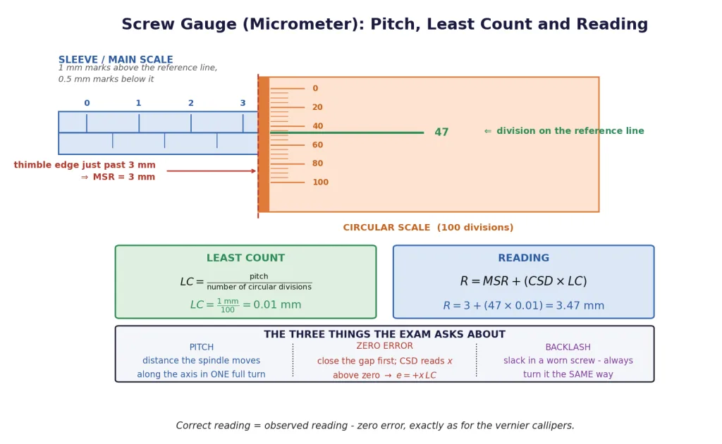
Key Point (Definition): The pitch of a screw gauge is the linear distance moved by the screw (spindle) along its axis in one complete rotation of the circular scale.

In practice you measure it by giving the thimble a known number of full turns and reading how far the edge advanced:

$$\text{pitch} = \frac{\text{distance moved on the main scale}}{\text{number of complete rotations}}$$

If the spindle advances 1 mm in 2 complete rotations, the pitch is 0.5 mm.

Least count

Key Point (Definition): $$LC = \frac{\text{pitch}}{\text{number of divisions on the circular scale}}$$

Pitch	Circular divisions	Least count
1 mm	100	0.01 mm $= 0.001$ cm
0.5 mm	50	0.01 mm $= 0.001$ cm
1 mm	50	0.02 mm $= 0.002$ cm
0.5 mm	100	0.005 mm

Notice the first two rows: halving the pitch and halving the number of divisions leaves the least count unchanged. Examiners love that.

Taking a reading

Key Point: $$\text{Reading} = MSR + (n \times LC)$$ where MSR is the main (pitch) scale reading visible just before the edge of the thimble, and $n$ is the circular scale division lying on the reference line.

The formula looks identical to the vernier's, but note the difference in what $n$ means: on a vernier you hunt for the division that coincides with a main mark; on a screw gauge you simply read off the division sitting on the reference line.

Zero error

Close the gap by rotating until the spindle just touches the anvil (use the safety ratchet — over-tightening distorts the reading and the instrument).

Key Point: If the circular scale zero lies below the reference line, so that the $x$-th division is on the line, the zero error is positive, $e = +x \times LC$. If the zero lies above the reference line with the $x$-th division on it, the zero error is negative, $e = -(N - x) \times LC$.

$$\text{Correct reading} = \text{Observed reading} - (\text{zero error})$$

Exactly the same correction rule as the vernier.

Backlash error

Key Point (Definition): Backlash error arises from wear and slack (play) between the screw and the nut. When the direction of rotation is reversed, the screw does not begin to advance immediately — the thimble turns through a little angle before the spindle moves at all.

Key Point (Remedy): Always rotate the screw in the same direction while taking a set of readings. If you must reverse, take up the slack first by turning well past the point and approaching again from the original direction.

Can you make it arbitrarily accurate?

Tempting: just cut 1000 divisions on the circular scale and get $LC = 0.001$ mm. It does not work.

Key Point: Increasing the number of circular divisions raises precision, not accuracy. Beyond a point, the reading is limited by physical realities the scale cannot fix — the elastic deformation of the object under the spindle's pressure, thermal expansion, backlash, and the finite thickness of the ruling itself. Precision without accuracy buys you nothing.

[Important] Both instruments follow the same three-line recipe: find LC, take the reading as $MSR + n \times LC$, then subtract the zero error. Get those three lines down and this entire topic is free marks.

Advanced Dimensional Analysis: Beyond Mechanics

Section 4 built dimensional formulae for mechanical quantities out of $[M]$, $[L]$ and $[T]$. JEE goes much further, into the four base dimensions that section left idling: electric current $[A]$, temperature $[K]$, amount of substance $[mol]$ and luminous intensity $[cd]$.

The recipe has not changed one bit — write the defining equation, substitute, collect powers. Only the equations are new.

Electrical and magnetic quantities

Quantity	Defining relation	Dimensional formula	SI unit
Electric charge $q$	$q = It$	$[\mathrm{M^0\,L^0\,T\,A}]$	coulomb (C)
Current density $J$	$J = \dfrac{I}{A}$	$[\mathrm{M^0\,L^{-2}\,T^0\,A}]$	$\mathrm{A\ m^{-2}}$
Potential, emf $V$	$V = \dfrac{W}{q}$	$[\mathrm{M\,L^2\,T^{-3}\,A^{-1}}]$	volt (V)
Electric field $E$	$E = \dfrac{F}{q}$	$[\mathrm{M\,L\,T^{-3}\,A^{-1}}]$	$\mathrm{V\ m^{-1}}$
Resistance $R$	$R = \dfrac{V}{I}$	$[\mathrm{M\,L^2\,T^{-3}\,A^{-2}}]$	ohm $(\Omega)$
Resistivity $\rho$	$\rho = \dfrac{RA}{l}$	$[\mathrm{M\,L^3\,T^{-3}\,A^{-2}}]$	$\Omega$ m
Capacitance $C$	$C = \dfrac{q}{V}$	$[\mathrm{M^{-1}\,L^{-2}\,T^{4}\,A^{2}}]$	farad (F)
Permittivity $\varepsilon_0$	$F = \dfrac{q_1 q_2}{4\pi\varepsilon_0 r^2}$	$[\mathrm{M^{-1}\,L^{-3}\,T^{4}\,A^{2}}]$	$\mathrm{C^2\ N^{-1}\ m^{-2}}$
Permeability $\mu_0$	$c^2 = \dfrac{1}{\mu_0 \varepsilon_0}$	$[\mathrm{M\,L\,T^{-2}\,A^{-2}}]$	$\mathrm{T\ m\ A^{-1}}$
Magnetic field $B$	$F = qvB$	$[\mathrm{M\,L^0\,T^{-2}\,A^{-1}}]$	tesla (T)
Magnetic flux $\phi$	$\phi = BA$	$[\mathrm{M\,L^2\,T^{-2}\,A^{-1}}]$	weber (Wb)
Self-inductance $L$	$\varepsilon = -L\dfrac{dI}{dt}$	$[\mathrm{M\,L^2\,T^{-2}\,A^{-2}}]$	henry (H)

Two derivations worth doing yourself right now, because everything electrical follows from them:

$$[V] = \frac{[W]}{[q]} = \frac{[\mathrm{M\,L^2\,T^{-2}}]}{[\mathrm{T\,A}]} = [\mathrm{M\,L^2\,T^{-3}\,A^{-1}}]$$

$$[R] = \frac{[V]}{[I]} = \frac{[\mathrm{M\,L^2\,T^{-3}\,A^{-1}}]}{[\mathrm{A}]} = [\mathrm{M\,L^2\,T^{-3}\,A^{-2}}]$$

Thermal quantities

Quantity	Defining relation	Dimensional formula	SI unit
Heat $Q$	a form of energy	$[\mathrm{M\,L^2\,T^{-2}}]$	joule (J)
Specific heat capacity $c$	$Q = mc\,\Delta T$	$[\mathrm{M^0\,L^2\,T^{-2}\,K^{-1}}]$	$\mathrm{J\ kg^{-1}\ K^{-1}}$
Latent heat $L$	$Q = mL$	$[\mathrm{M^0\,L^2\,T^{-2}}]$	$\mathrm{J\ kg^{-1}}$
Heat capacity, entropy	$S = \dfrac{Q}{T}$	$[\mathrm{M\,L^2\,T^{-2}\,K^{-1}}]$	$\mathrm{J\ K^{-1}}$
Thermal conductivity $K$	$Q = KA\dfrac{\Delta T}{\Delta x}t$	$[\mathrm{M\,L\,T^{-3}\,K^{-1}}]$	$\mathrm{W\ m^{-1}\ K^{-1}}$
Gas constant $R$	$PV = nRT$	$[\mathrm{M\,L^2\,T^{-2}\,K^{-1}\,mol^{-1}}]$	$\mathrm{J\ mol^{-1}\ K^{-1}}$
Boltzmann constant $k$	$PV = NkT$	$[\mathrm{M\,L^2\,T^{-2}\,K^{-1}}]$	$\mathrm{J\ K^{-1}}$
Coefficient of linear expansion $\alpha$	$\alpha = \dfrac{\Delta L}{L\,\Delta T}$	$[\mathrm{M^0\,L^0\,T^0\,K^{-1}}]$	$\mathrm{K^{-1}}$

Note the pair of constants: $R$ is per mole, $k$ is per molecule, and $N$ in $PV = NkT$ is a pure count. So $R$ and $k$ differ by exactly one factor of $[\mathrm{mol^{-1}}]$ — and $kT$ has the dimensions of energy, which is the fastest way to remember $k$ at all.

Modern-physics constants

Quantity	Defining relation	Dimensional formula	SI unit
Planck constant $h$	$E = h\nu$	$[\mathrm{M\,L^2\,T^{-1}}]$	J s
Stefan constant $\sigma$	$\dfrac{E}{At} = \sigma T^4$	$[\mathrm{M\,L^0\,T^{-3}\,K^{-4}}]$	$\mathrm{W\ m^{-2}\ K^{-4}}$
Wien constant $b$	$\lambda_m T = b$	$[\mathrm{M^0\,L\,T^0\,K}]$	m K
Work function $\phi_0$	an energy	$[\mathrm{M\,L^2\,T^{-2}}]$	J (or eV)
Rydberg constant $R_H$	$\dfrac{1}{\lambda} = R_H(\ldots)$	$[\mathrm{M^0\,L^{-1}\,T^0}]$	$\mathrm{m^{-1}}$
Decay constant $\lambda$	$N = N_0 e^{-\lambda t}$	$[\mathrm{M^0\,L^0\,T^{-1}}]$	$\mathrm{s^{-1}}$

Finding unknown exponents in a given relation

A standing favourite: you are told a quantity is built from certain others, and asked for the powers.

Worked case. The energy density $u$ of a magnetic field is known to be of the form $u = B^a \mu_0^{\,b}$. Find $a$ and $b$.

1. Write every dimensional formula. $[u] = \dfrac{[\text{energy}]}{[\text{volume}]} = [\mathrm{M\,L^{-1}\,T^{-2}}]$, $[B] = [\mathrm{M\,T^{-2}\,A^{-1}}]$, $[\mu_0] = [\mathrm{M\,L\,T^{-2}\,A^{-2}}]$.
2. Substitute and collect. $$[\mathrm{M\,L^{-1}\,T^{-2}}] = [\mathrm{M\,T^{-2}\,A^{-1}}]^a\,[\mathrm{M\,L\,T^{-2}\,A^{-2}}]^b = [\mathrm{M^{a+b}\,L^{b}\,T^{-2a-2b}\,A^{-a-2b}}]$$
3. Equate powers, one base quantity at a time.

• $L$: $\;b = -1$
• $M$: $\;a + b = 1 \Rightarrow a = 2$
• Check $T$: $-2(2) - 2(-1) = -2$. Correct.
• Check $A$: $-(2) - 2(-1) = 0$. Correct.

1. Conclude: $a = 2$, $b = -1$, so $u = \dfrac{B^2}{\mu_0}$ — which is indeed the standard result (with a $\frac{1}{2}$ out front that dimensions can never see).

Key Point (the method): Equate the powers of $M$, $L$, $T$, $A$ and $K$ separately. You get one linear equation per base quantity, and any that you did not need become free checks on your answer.

Pairs with identical dimensions

The single highest-frequency question type in the chapter. Section 4 gave you the mechanical groups; here is the full list.

Group of quantities	Common dimensional formula
impulse, linear momentum	$[\mathrm{M\,L\,T^{-1}}]$
work, energy, torque, heat, moment of force	$[\mathrm{M\,L^2\,T^{-2}}]$
pressure, stress, Young's modulus, bulk modulus, energy density	$[\mathrm{M\,L^{-1}\,T^{-2}}]$
Planck constant, angular momentum	$[\mathrm{M\,L^2\,T^{-1}}]$
surface tension, spring constant, surface energy per unit area	$[\mathrm{M\,L^0\,T^{-2}}]$
frequency, angular velocity, velocity gradient, decay constant	$[\mathrm{M^0\,L^0\,T^{-1}}]$
latent heat, gravitational potential, (velocity)$^2$	$[\mathrm{M^0\,L^2\,T^{-2}}]$
Boltzmann constant, entropy, heat capacity	$[\mathrm{M\,L^2\,T^{-2}\,K^{-1}}]$
magnetic flux, $h/e$	$[\mathrm{M\,L^2\,T^{-2}\,A^{-1}}]$
$\dfrac{L}{R}$, $RC$, $\sqrt{LC}$, time period	$[\mathrm{M^0\,L^0\,T}]$

That last row is worth its own line, because circuit problems lean on it constantly:

$$\left[\frac{L}{R}\right] = \frac{[\mathrm{M\,L^2\,T^{-2}\,A^{-2}}]}{[\mathrm{M\,L^2\,T^{-3}\,A^{-2}}]} = [\mathrm{T}], \qquad [RC] = [\mathrm{M\,L^2\,T^{-3}\,A^{-2}}][\mathrm{M^{-1}\,L^{-2}\,T^{4}\,A^{2}}] = [\mathrm{T}]$$

Key Point: Identical dimensions still do not mean identical quantities. Work and torque share a formula and are different physics; the Planck constant and angular momentum share a formula, which turns out to be why angular momentum is quantised in units of $\hbar$. Dimensions record the recipe, never the meaning.

[Advanced] The genuinely hard version of this question hands you a composite expression and asks what it matches — for example $\varepsilon_0 L \dfrac{\Delta V}{\Delta t}$, or $\dfrac{e^2}{4\pi\varepsilon_0 \hbar c}$. Do not guess. Substitute from the tables above and grind the exponents out; both are done in the solved examples.

Solved Examples

Example 1: Mean absolute error, relative error and percentage error

The period of oscillation of a simple pendulum is measured five times with a stopwatch and the readings are 2.63 s, 2.56 s, 2.42 s, 2.71 s and 2.80 s. Calculate the mean period, the mean absolute error, the relative error and the percentage error, and quote the result properly.

Solution:

1. Mean value. Add the five readings and divide by 5: $$T_{mean} = \frac{2.63 + 2.56 + 2.42 + 2.71 + 2.80}{5} = \frac{13.12}{5} = 2.624\ \text{s}$$ The readings are given to two decimal places, so we keep the mean to the same precision: $T_{mean} = 2.62$ s.
2. Absolute error of every reading, as a magnitude:

Reading (s)	$\Delta T_i = T_{mean} - T_i$	$\vert\Delta T_i\vert$ (s)
2.63	$-0.01$	0.01
2.56	$+0.06$	0.06
2.42	$+0.20$	0.20
2.71	$-0.09$	0.09
2.80	$-0.18$	0.18

3. Mean absolute error. Add the magnitudes and divide by 5: $$\Delta T_{mean} = \frac{0.01 + 0.06 + 0.20 + 0.09 + 0.18}{5} = \frac{0.54}{5} = 0.108 \approx 0.11\ \text{s}$$
4. Report the result. $T = 2.62 \pm 0.11$ s. Any single measurement of the period is likely to lie between 2.51 s and 2.73 s.
5. Relative error. $$\frac{\Delta T_{mean}}{T_{mean}} = \frac{0.11}{2.62} = 0.042$$
6. Percentage error. $\delta T = 0.042 \times 100 = 4.2\%$, usually quoted as 4%.

Final Answer: $T = 2.62 \pm 0.11$ s, relative error 0.04, percentage error about 4%.

Takeaway: Take the magnitudes before averaging. If you average the signed deviations you get $(-0.01 + 0.06 + 0.20 - 0.09 - 0.18)/5 \approx 0$, which is true and completely useless — it is exactly the cancellation that makes the mean a good estimate in the first place.

Example 2: Why differences are dangerous

Two temperatures are measured with the same thermometer as $t_1 = 25.0 \pm 0.5\ ^\circ$C and $t_2 = 20.0 \pm 0.5\ ^\circ$C. Find the temperature difference with its error, and compare the percentage errors.

Solution:

1. Percentage error of each reading. $$\delta t_1 = \frac{0.5}{25.0}\times 100 = 2.0\%, \qquad \delta t_2 = \frac{0.5}{20.0}\times 100 = 2.5\%$$ Both are perfectly respectable measurements.
2. The difference. $t_1 - t_2 = 25.0 - 20.0 = 5.0\ ^\circ$C.
3. Its absolute error — Rule 2, the errors ADD: $$\Delta(t_1 - t_2) = \Delta t_1 + \Delta t_2 = 0.5 + 0.5 = 1.0\ ^\circ\text{C}$$
4. Percentage error of the difference. $$\frac{1.0}{5.0}\times 100 = 20\%$$

Final Answer: $\Delta t = 5.0 \pm 1.0\ ^\circ$C, a percentage error of 20%.

Takeaway: Two 2%-quality measurements produced a 20%-quality answer. The absolute error stayed at 1.0 while the result shrank from 25 to 5 — that is the whole mechanism. Whenever an experiment can be redesigned to measure a difference directly instead of subtracting two large numbers, redesign it.

Example 3: Resistors in parallel [Advanced]

Two resistors $R_1 = 100 \pm 3\ \Omega$ and $R_2 = 200 \pm 4\ \Omega$ are connected (a) in series and (b) in parallel. Find the equivalent resistance with its error in each case.

Solution:

1. (a) Series: $R = R_1 + R_2 = 100 + 200 = 300\ \Omega$. By Rule 1 the absolute errors add: $$\Delta R = \Delta R_1 + \Delta R_2 = 3 + 4 = 7\ \Omega \quad \Rightarrow \quad R = 300 \pm 7\ \Omega$$
2. (b) Parallel: $\dfrac{1}{R} = \dfrac{1}{R_1} + \dfrac{1}{R_2} = \dfrac{1}{100} + \dfrac{1}{200} = \dfrac{3}{200}$, so $R = \dfrac{200}{3} = 66.7\ \Omega$.
3. Propagate the error. Differentiating the reciprocal relation, $\dfrac{\Delta R}{R^2} = \dfrac{\Delta R_1}{R_1^2} + \dfrac{\Delta R_2}{R_2^2}$, so $$\Delta R = R^2\left(\frac{\Delta R_1}{R_1^2} + \frac{\Delta R_2}{R_2^2}\right)$$
4. Substitute. $$\Delta R = (66.7)^2\left(\frac{3}{100^2} + \frac{4}{200^2}\right) = 4444.4 \times (0.0003 + 0.0001) = 4444.4 \times 0.0004 = 1.8\ \Omega$$

Final Answer: Series $R = 300 \pm 7\ \Omega$; parallel $R = 66.7 \pm 1.8\ \Omega$.

Takeaway: For anything shaped like $1/R$, propagate the reciprocal first and convert back at the end — do not try to apply the product rule to the original expression. Note also that the parallel combination has the smaller absolute error, but its percentage error ($1.8/66.7 = 2.7$%) is larger than the series one ($7/300 = 2.3$%).

Example 4: Percentage error in density from mass and diameter

The density of a solid sphere is found by measuring its mass and its diameter. If the percentage error in the mass is 1.5% and in the diameter is 2%, find the maximum percentage error in the calculated density.

Solution:

1. Write the formula and expose every power. $\rho = \dfrac{m}{V}$ and $V = \dfrac{4}{3}\pi r^3 = \dfrac{\pi}{6}d^3$, so $$\rho = \frac{6m}{\pi d^3} = \frac{6}{\pi}\, m\, d^{-3}$$ The factor $6/\pi$ is a pure number and contributes nothing.
2. Apply Rule 4. The powers are 1 for $m$ and 3 for $d$ (magnitude of the exponent): $$\frac{\Delta \rho}{\rho} = \frac{\Delta m}{m} + 3\,\frac{\Delta d}{d}$$
3. Substitute the percentages. $$\delta\rho = 1.5 + 3(2) = 1.5 + 6 = 7.5\%$$

Final Answer: The maximum error in the density is 7.5%.

Takeaway: The diameter was measured only slightly worse than the mass, but it entered cubed and so supplied 6 of the 7.5 percentage points — 80% of the error budget. If you get one more shot at improving this experiment, you spend it on the diameter.

Example 5: Numerical version with real readings

A sphere has mass $22.42 \pm 0.01$ g and diameter $2.50 \pm 0.01$ cm. Find its density and the percentage error in it.

Solution:

1. Percentage error in mass. $\dfrac{0.01}{22.42}\times 100 = 0.045\%$.
2. Percentage error in diameter. $\dfrac{0.01}{2.50}\times 100 = 0.4\%$.
3. Combine, remembering the cube: $$\delta\rho = 0.045 + 3(0.4) = 0.045 + 1.2 = 1.2\%$$
4. The density itself. $V = \dfrac{\pi}{6}(2.50)^3 = \dfrac{\pi}{6}(15.625) = 8.18\ \text{cm}^3$, so $$\rho = \frac{22.42}{8.18} = 2.74\ \text{g cm}^{-3}$$

Final Answer: $\rho = 2.74$ g cm$^{-3}$ with a percentage error of about 1.2%.

Takeaway: The mass was measured to a spectacular 0.045% and it contributed almost nothing. A cube in the formula turns a modest 0.4% into 1.2%. Powers, not raw errors, decide who matters.

Example 6: Accuracy of $g$ from a pendulum experiment

The period of a simple pendulum is $T = 2\pi\sqrt{L/g}$. The measured length is 20.0 cm known to 1 mm accuracy, and the time for 100 oscillations is 90 s measured with a wrist watch of 1 s resolution. What is the accuracy in the determination of $g$?

Solution:

1. Make $g$ the subject. Squaring, $T^2 = \dfrac{4\pi^2 L}{g}$, so $$g = \frac{4\pi^2 L}{T^2}$$
2. Identify the powers. $L$ appears to the power 1, $T$ to the power 2; $4\pi^2$ is a pure number. So $$\frac{\Delta g}{g} = \frac{\Delta L}{L} + 2\,\frac{\Delta T}{T}$$
3. The length term. $\Delta L$ is the least count, 1 mm $= 0.1$ cm: $$\frac{\Delta L}{L} = \frac{0.1}{20.0} = 0.005$$
4. The time term — this is the step that is worth the marks. We measured $t = 90$ s for $n = 100$ oscillations, so $T = t/n$. The number 100 is an exact counted number with no error at all, so $$\frac{\Delta T}{T} = \frac{\Delta t / n}{t / n} = \frac{\Delta t}{t} = \frac{1}{90} = 0.0111$$
5. Combine. $$\frac{\Delta g}{g} = 0.005 + 2(0.0111) = 0.005 + 0.0222 = 0.0272$$
6. As a percentage: $0.0272 \times 100 = 2.72\%$, which we round to 3%.

Final Answer: The accuracy in $g$ is about $\pm 2.7\%$, i.e. roughly 3%.

Takeaway: Timing 100 oscillations instead of 1 divided the relative error in $T$ by 100 — the single most valuable trick in the whole practical syllabus, and the reason $n$ being exact matters. Even so, the time term still contributes 2.2 of the 2.7 percentage points, because of the square.

Example 7: Error in Young's modulus [Advanced]

Young's modulus of a wire is measured using $Y = \dfrac{MgL}{\pi r^2 e}$, where $M$ is the suspended mass, $L$ the wire's length, $r$ its radius and $e$ its extension. The measurements are $M = 5.00 \pm 0.05$ kg, $L = 2.000 \pm 0.001$ m, $r = 0.500 \pm 0.005$ mm and $e = 0.80 \pm 0.05$ mm. Find the maximum percentage error in $Y$, and identify which measurement should be improved first.

Solution:

1. Rewrite with explicit powers. $g$ and $\pi$ are constants, so $$Y \propto M^{1} L^{1} r^{-2} e^{-1} \quad \Rightarrow \quad \frac{\Delta Y}{Y} = \frac{\Delta M}{M} + \frac{\Delta L}{L} + 2\frac{\Delta r}{r} + \frac{\Delta e}{e}$$ Note the 2 on the radius term — and note that $r$ and $e$ sitting in the denominator makes no difference to the sign.
2. Compute each term as a percentage.

Quantity	Value	$\Delta$	Power	Contribution
$M$	5.00 kg	0.05 kg	1	$1 \times \frac{0.05}{5.00}\times 100 = 1.00$%
$L$	2.000 m	0.001 m	1	$1 \times \frac{0.001}{2.000}\times 100 = 0.05$%
$r$	0.500 mm	0.005 mm	2	$2 \times \frac{0.005}{0.500}\times 100 = 2.00$%
$e$	0.80 mm	0.05 mm	1	$1 \times \frac{0.05}{0.80}\times 100 = 6.25$%

3. Add them all — errors never cancel. $$\delta Y = 1.00 + 0.05 + 2.00 + 6.25 = 9.30\%$$

Final Answer: The maximum percentage error in $Y$ is 9.3%, and the extension $e$ is by far the worst offender at 6.25 of those 9.3 percentage points.

Takeaway: The extension has only the power 1, yet it dominates — because it is a tiny quantity (0.80 mm) measured with a comparatively coarse uncertainty. Power is not the only thing that matters; relative size matters too. The fix is to hang a bigger mass so that $e$ becomes larger and $\Delta e/e$ falls.

Example 8: Which measurement deserves the most care? [Advanced]

A quantity is calculated as $Z = \dfrac{A^2 B^{1/2}}{C^{1/3} D^3}$. The percentage errors in $A$, $B$, $C$ and $D$ are 1%, 2%, 3% and 0.5% respectively. Find the maximum percentage error in $Z$, and state which measurement you should improve first.

Solution:

1. Write the propagation rule, taking the magnitude of every exponent. $$\frac{\Delta Z}{Z} = 2\frac{\Delta A}{A} + \frac{1}{2}\frac{\Delta B}{B} + \frac{1}{3}\frac{\Delta C}{C} + 3\frac{\Delta D}{D}$$
2. Evaluate every contribution separately — this table is the answer to the second half of the question:

Quantity	Power	Percentage error	Contribution
$A$	2	1%	2.0%
$B$	$1/2$	2%	1.0%
$C$	$1/3$	3%	1.0%
$D$	3	0.5%	1.5%

3. Total: $$\delta Z = 2.0 + 1.0 + 1.0 + 1.5 = 5.5\%$$

Final Answer: $\delta Z = 5.5\%$, and $A$ contributes the most (2.0%), so $A$ should be measured most carefully.

Takeaway: $C$ is the sloppiest measurement at 3% and contributes the least, because its exponent is only $1/3$. $A$ is one of the tidiest and contributes the most, because it is squared. Always rank by power $\times$ error, never by error alone — that comparison is exactly what this question type is testing.

Example 9: Vernier callipers — least count, reading and zero error

A vernier calliper has a main scale graduated in millimetres, with 10 vernier divisions coinciding with 9 main scale divisions. With the jaws fully closed, the 4th vernier division coincides with a main scale division. While measuring a rod, the main scale reads 4.2 cm and the 6th vernier division coincides with a main scale mark. Find (a) the least count, (b) the observed reading, (c) the zero error and (d) the correct length.

Solution:

1. (a) Least count. 10 vernier divisions $=$ 9 main divisions, so $N = 10$ and $1\ MSD = 1$ mm: $$LC = \frac{MSD}{N} = \frac{1\ \text{mm}}{10} = 0.1\ \text{mm} = 0.01\ \text{cm}$$
2. (b) Observed reading. The 6th vernier division coincides, so $$R_{obs} = MSR + (n \times LC) = 4.2 + (6 \times 0.01) = 4.2 + 0.06 = 4.26\ \text{cm}$$
3. (c) Zero error. With the jaws closed the vernier zero has drifted to the right of the main zero (the 4th division coincides on the positive side), so the zero error is positive: $$e = +4 \times 0.01 = +0.04\ \text{cm}$$
4. (d) Correct reading. Always $\text{correct} = \text{observed} - e$: $$L = 4.26 - (+0.04) = 4.22\ \text{cm}$$

Final Answer: $LC = 0.01$ cm, observed 4.26 cm, zero error $+0.04$ cm, correct length 4.22 cm.

Takeaway: A positive zero error means the instrument was reading too high, so you subtract. Had the same calliper shown a negative zero error with the 6th division coinciding, it would have been $e = -(10 - 6)\times 0.01 = -0.04$ cm, and the correct length would have been $4.26 - (-0.04) = 4.30$ cm — larger, not smaller.

Example 10: Screw gauge — least count, reading, zero error and percentage error

The pitch of a screw gauge is 1 mm and its circular scale carries 100 divisions. When the gap is closed the circular scale reads 5 divisions above its zero. While measuring the diameter of a wire the main scale reads 3 mm and the 47th circular division lies on the reference line. Find the least count, the corrected diameter, and the percentage error in the cross-sectional area of the wire.

Solution:

1. Least count. $$LC = \frac{\text{pitch}}{\text{number of circular divisions}} = \frac{1\ \text{mm}}{100} = 0.01\ \text{mm}$$
2. Observed reading. $$R_{obs} = MSR + (n \times LC) = 3 + (47 \times 0.01) = 3 + 0.47 = 3.47\ \text{mm}$$
3. Zero error and correction. The zero of the circular scale is 5 divisions past the reference line, a positive zero error $e = +5 \times 0.01 = +0.05$ mm: $$d = 3.47 - (+0.05) = 3.42\ \text{mm}$$
4. Percentage error in $d$. The uncertainty in a single reading is the least count: $$\frac{\Delta d}{d}\times 100 = \frac{0.01}{3.42}\times 100 = 0.29\%$$
5. Percentage error in the area. $A = \dfrac{\pi d^2}{4} \propto d^2$, so the exponent 2 doubles it: $$\delta A = 2 \times 0.29 = 0.58\%$$

Final Answer: $LC = 0.01$ mm, corrected diameter $d = 3.42$ mm, and the area carries about 0.58% error.

Takeaway: Three lines, every time: least count, then $MSR + n \times LC$, then subtract the zero error. And once you have a diameter, remember that anything built on $d^2$ (area) or $d^3$ (volume, density) doubles or trebles its percentage error.

Example 11: Dimensional formulae of electrical quantities

Derive the dimensional formulae of (i) electric charge, (ii) electric potential, (iii) resistance, (iv) capacitance and (v) the permittivity of free space $\varepsilon_0$.

Solution:

1. (i) Charge. $q = It$, so $$[q] = [\mathrm{A}][\mathrm{T}] = [\mathrm{M^0\,L^0\,T\,A}]$$
2. (ii) Potential. $V = \dfrac{W}{q}$, and work is $[\mathrm{M\,L^2\,T^{-2}}]$: $$[V] = \frac{[\mathrm{M\,L^2\,T^{-2}}]}{[\mathrm{T\,A}]} = [\mathrm{M\,L^2\,T^{-3}\,A^{-1}}]$$
3. (iii) Resistance. From Ohm's law $R = \dfrac{V}{I}$: $$[R] = \frac{[\mathrm{M\,L^2\,T^{-3}\,A^{-1}}]}{[\mathrm{A}]} = [\mathrm{M\,L^2\,T^{-3}\,A^{-2}}]$$
4. (iv) Capacitance. $C = \dfrac{q}{V}$: $$[C] = \frac{[\mathrm{T\,A}]}{[\mathrm{M\,L^2\,T^{-3}\,A^{-1}}]} = [\mathrm{M^{-1}\,L^{-2}\,T^{4}\,A^{2}}]$$ Check the time exponent: $1 - (-3) = 4$. Check the current exponent: $1 - (-1) = 2$.
5. (v) Permittivity. From Coulomb's law $F = \dfrac{q_1 q_2}{4\pi\varepsilon_0 r^2}$, rearranged as $\varepsilon_0 = \dfrac{q_1 q_2}{4\pi F r^2}$: $$[\varepsilon_0] = \frac{[\mathrm{T\,A}]^2}{[\mathrm{M\,L\,T^{-2}}][\mathrm{L^2}]} = \frac{[\mathrm{T^2\,A^2}]}{[\mathrm{M\,L^3\,T^{-2}}]} = [\mathrm{M^{-1}\,L^{-3}\,T^{4}\,A^{2}}]$$

Final Answer: $[q] = [\mathrm{T\,A}]$, $[V] = [\mathrm{M\,L^2\,T^{-3}\,A^{-1}}]$, $[R] = [\mathrm{M\,L^2\,T^{-3}\,A^{-2}}]$, $[C] = [\mathrm{M^{-1}\,L^{-2}\,T^{4}\,A^{2}}]$, $[\varepsilon_0] = [\mathrm{M^{-1}\,L^{-3}\,T^{4}\,A^{2}}]$.

Takeaway: Everything electrical is a two-step chain off work and charge. Learn $[V]$ properly and the rest — $R$, $C$, $E$, $\varepsilon_0$ — falls out in one line each. Notice too that $[\varepsilon_0]$ and $[C]$ differ by exactly one power of length, which is why a capacitance is always $\varepsilon_0 \times$ (a length).

Example 12: The composite-expression question [Advanced]

(a) A quantity $X$ is given by $X = \varepsilon_0 L \dfrac{\Delta V}{\Delta t}$, where $\varepsilon_0$ is the permittivity of free space, $L$ a length, $\Delta V$ a potential difference and $\Delta t$ a time interval. Find the dimensional formula of $X$ and name the quantity it matches. (b) Show that $\dfrac{L}{R}$ and $RC$ both have the dimensions of time.

Solution:

1. (a) Write down each piece. $[\varepsilon_0] = [\mathrm{M^{-1}\,L^{-3}\,T^{4}\,A^{2}}]$, $[L] = [\mathrm{L}]$, and $$\left[\frac{\Delta V}{\Delta t}\right] = \frac{[\mathrm{M\,L^2\,T^{-3}\,A^{-1}}]}{[\mathrm{T}]} = [\mathrm{M\,L^2\,T^{-4}\,A^{-1}}]$$
2. Multiply and collect one base quantity at a time.

• $M$: $-1 + 0 + 1 = 0$
• $L$: $-3 + 1 + 2 = 0$
• $T$: $+4 + 0 - 4 = 0$
• $A$: $+2 + 0 - 1 = +1$

1. Therefore $[X] = [\mathrm{M^0\,L^0\,T^0\,A}] = [\mathrm{A}]$ — the dimensions of electric current.
2. (b) The inductive time constant. With $[L_{ind}] = [\mathrm{M\,L^2\,T^{-2}\,A^{-2}}]$ and $[R] = [\mathrm{M\,L^2\,T^{-3}\,A^{-2}}]$: $$\left[\frac{L_{ind}}{R}\right] = \frac{[\mathrm{M\,L^2\,T^{-2}\,A^{-2}}]}{[\mathrm{M\,L^2\,T^{-3}\,A^{-2}}]} = [\mathrm{T}]$$ Every exponent cancels except time, where $-2 - (-3) = +1$.
3. The capacitive time constant. $$[RC] = [\mathrm{M\,L^2\,T^{-3}\,A^{-2}}] \times [\mathrm{M^{-1}\,L^{-2}\,T^{4}\,A^{2}}] = [\mathrm{M^0\,L^0\,T\,A^0}] = [\mathrm{T}]$$

Final Answer: (a) $[X] = [\mathrm{A}]$, the dimensions of electric current. (b) Both $L/R$ and $RC$ have dimensions $[\mathrm{M^0\,L^0\,T}]$.

Takeaway: $X$ here is physically the displacement current of Maxwell's equations, and the dimensional check is the fastest possible confirmation. For part (b), $\sqrt{LC}$ is a time as well — which is why $\omega = 1/\sqrt{LC}$ is a frequency. Never guess on these: line up the exponents of $M$, $L$, $T$ and $A$ in a column and add.