Ampere's Circuital Law

Stating Ampère's Circuital Law

The Biot-Savart law of Section 5 gives us a complete recipe for computing the magnetic field of any steady current distribution — in principle. But for most non-trivial geometries, the integration is painful. We need a smarter tool.

That tool is Ampère's circuital law, the magnetic analogue of Gauss's law in electrostatics. It exploits symmetry to shortcut the integration.

Note: In this form, Ampère's law assumes steady currents only (magnetostatics). When currents vary with time, Maxwell's displacement current term must be added (leading to the Ampère–Maxwell law).

Statement

For any closed loop drawn in space, the line integral of the magnetic field around the loop equals $\mu_0$ times the total current that passes through (is enclosed by) the loop.

In symbols:

$$\boxed{\;\oint \vec{B}\cdot d\vec{l} = \mu_0\,I_{enc}\;}$$

A few terminology notes:

• The closed loop is called an Amperian loop. It is imaginary — you draw it strategically, wherever the symmetry is convenient.
• $I_{enc}$ is the net current enclosed: currents going one way are positive, currents going the other way are negative (sign by right-hand rule).
• The equation holds for any closed loop in space, but it's only useful for computing $\vec{B}$ when symmetry lets you argue that $|\vec{B}|$ has constant magnitude and a known direction on the loop.

Sign Convention and When to Use Ampère's Law

Sign convention — right-hand rule

To assign signs to enclosed currents:

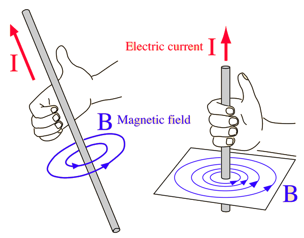
Curl the fingers of your right hand along $d\vec{l}$ (the direction you traverse the Amperian loop). Your thumb then defines the positive sense for $I_{enc}$. Currents flowing along the thumb count as positive; currents flowing opposite to the thumb count as negative.

When we say “counter-clockwise as seen from above,” we mean: look along the direction of your thumb and view the plane of the loop; if your fingers curl counter-clockwise in that view, then currents pointing toward you (out of the page) are positive.

When does Ampère's law actually help?

The law is always true, but to use it as a computational tool you need a geometry where:

1. The magnetic field magnitude $|\vec{B}|$ is constant at every point on the Amperian loop, and
2. The angle between $\vec{B}$ and $d\vec{l}$ is constant (usually $0^\circ$ or $90^\circ$) everywhere on the loop.

When those two conditions are met, $\displaystyle\oint \vec{B}\cdot d\vec{l} = B\times$(length of loop), and you can solve algebraically for $B$.

The four classic Ampère-friendly geometries

Geometry	Amperian loop	Outcome
Long straight wire	Circle around the wire	$B = \mu_0 I / (2\pi r)$
Long thick cylindrical wire	Circle around the axis	Inside: $B = \mu_0 I r/(2\pi a^2)$ Outside: $B = \mu_0 I/(2\pi r)$
Solenoid	Rectangle straddling the coil walls	$B = \mu_0 n I$ inside
Toroid	Circle along a “meridian” inside	$B = \mu_0 N I/(2\pi r)$ inside

Application 1 — Long Straight Wire (Re-derivation)

We already know from Biot-Savart that $B = \mu_0 I/(2\pi a)$ for an infinite straight wire. Let's re-derive it from Ampère's law in three lines — much faster.

Geometry: Wire along the $z$-axis carrying current $I$ upward. By symmetry (rotational symmetry around the wire), the field magnitude $B$ depends only on perpendicular distance $r$, and is everywhere tangent to circles around the wire.

Amperian loop: A circle of radius $r$ centred on the wire, in a plane perpendicular to the wire, traversed counter-clockwise as viewed from above.

Compute the line integral: $\vec{B}\parallel d\vec{l}$ at every point on the circle, so $\vec{B}\cdot d\vec{l} = B\,dl$. Also $|\vec{B}|$ is constant on the circle:

$$\oint \vec{B}\cdot d\vec{l} = B\oint dl = B\cdot 2\pi r$$

Apply Ampère's law: $I_{enc} = I$ (the wire passes through the loop).

$$B\cdot 2\pi r = \mu_0 I \quad\Rightarrow\quad B = \dfrac{\mu_0 I}{2\pi r}$$

A three-line derivation that took us a calculus integral with Biot-Savart. Ampère's law is fast — when the geometry cooperates.

[JEE Tip] In any “derive $B$ of a long straight wire” question, the Ampère-law derivation is the expected method. Mention symmetry, draw the Amperian loop, and bring out $B$ from the integral.

Application 2 — Field of a Thick Cylindrical Wire

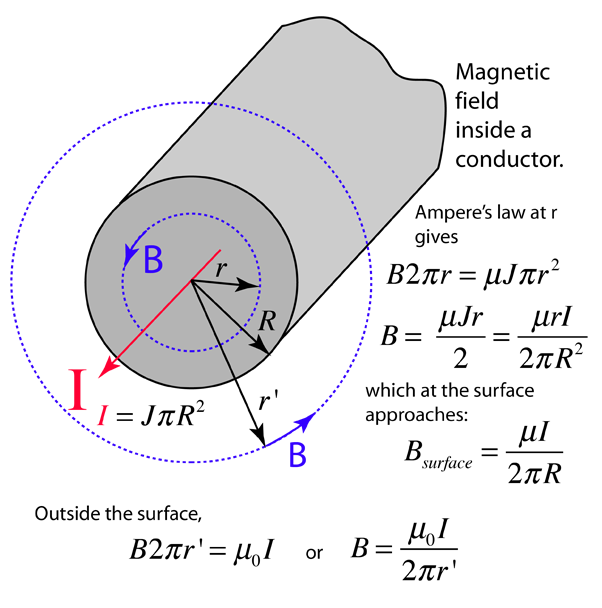
A real wire has a finite thickness. Consider a long cylindrical conductor of radius $a$ carrying a steady current $I$ distributed uniformly over its cross-section.

Current density definition: Let $J$ be the magnitude of the uniform current density (current per unit area).

$$J = \frac{I}{\pi a^2}$$

We want $\vec{B}$ at radial distance $r$ from the axis, both inside ($r < a$) and outside ($r > a$) the wire.

Outside the wire ($r > a$)

Use a circular Amperian loop of radius $r$ outside the wire. All the current $I$ is enclosed, and by symmetry $B$ is constant and tangent on the loop:

$$B(2\pi r) = \mu_0 I \quad\Rightarrow\quad B = \dfrac{\mu_0 I}{2\pi r}$$

Same as a thin wire — from outside, a thick wire looks just like a thin one.

Inside the wire ($r < a$)

Use a circular Amperian loop of radius $r$ inside the wire. Only the current passing through this smaller circle is enclosed:

$$I_{enc} = J\cdot \pi r^2 = \dfrac{I}{\pi a^2}\,\pi r^2 = \dfrac{I r^2}{a^2}$$

Apply Ampère's law:

$$B(2\pi r) = \mu_0\,\dfrac{I r^2}{a^2} \quad\Rightarrow\quad B = \dfrac{\mu_0 I r}{2\pi a^2}$$

Summary and graph

Region	Formula	Behaviour
$r < a$ (inside)	$B = \mu_0 I r/(2\pi a^2)$	Grows linearly from $0$ at axis
$r = a$ (surface)	$B = \mu_0 I/(2\pi a)$	Maximum value
$r > a$ (outside)	$B = \mu_0 I/(2\pi r)$	Falls as $1/r$

The field is zero on the axis, peaks at the surface, and falls off outside.

Coaxial cable note

A coaxial cable consists of a central conductor (radius $a$, current $I$ one way) inside a thin outer cylindrical shell (radius $b>a$, current $I$ the other way). Apply Ampère's law:

• $r < a$: $B = \mu_0 I r/(2\pi a^2)$
• $a < r < b$: $B = \mu_0 I/(2\pi r)$
• $r > b$: $B = 0$ (inner and outer currents cancel)

This is why coaxial cables have no external magnetic interference — they are self-shielded.

Memory Capsule

A compact summary to lock in.

Ampère's circuital law (memorise)

$$\oint \vec{B}\cdot d\vec{l} = \mu_0\,I_{enc}$$

• Loop is imaginary, chosen for symmetry.
• $I_{enc}$ is net current threading the loop, signed by right-hand rule.

When is it useful?

Only when symmetry guarantees:

1. $|\vec{B}|$ is constant on the loop, and
2. The angle between $\vec{B}$ and $d\vec{l}$ is constant.

Key results from this section

Geometry	Field
Long straight wire (any $r>0$)	$B = \mu_0 I/(2\pi r)$
Thick wire, inside ($r<a$)	$B = \mu_0 I r/(2\pi a^2)$
Thick wire, outside ($r>a$)	$B = \mu_0 I/(2\pi r)$
Coaxial cable, $a<r<b$	$B = \mu_0 I/(2\pi r)$
Coaxial cable, $r>b$	$B = 0$

One-line takeaway: Ampère's law is the magnetic Gauss's law: rewrite a calculus integral as one-line algebra whenever symmetry exists.

Solved Examples

Example 1: Straight-wire derivation, fast
State and use Ampère's circuital law to derive $B = \mu_0 I/(2\pi r)$ for a long straight wire.

Solution. Ampère's law: $\oint \vec{B}\cdot d\vec{l} = \mu_0 I_{enc}$.

Choose a circular Amperian loop of radius $r$ centred on the wire and perpendicular to it. By cylindrical symmetry, $\vec{B}$ is tangent to the loop everywhere and constant in magnitude. So

$$\oint \vec{B}\cdot d\vec{l} = B(2\pi r) = \mu_0 I$$ $$B = \dfrac{\mu_0 I}{2\pi r}$$

A 3-mark Board answer.

Example 2: Field inside a thick wire
A long straight cylindrical wire of radius $a = 2\text{ cm}$ carries a current of $I = 8\text{ A}$ distributed uniformly. Find $B$ at (a) $r = 1\text{ cm}$ and (b) $r = 4\text{ cm}$.

Solution.
(a) $r = 1\text{ cm}<2\text{ cm}$, inside formula: $$B = \dfrac{\mu_0 I r}{2\pi a^2} = \dfrac{(4\pi\times10^{-7})(8)(0.01)}{2\pi(0.02)^2} = 4\times10^{-5}\;\mathrm{T}$$

(b) $r = 4\text{ cm}>2\text{ cm}$, outside formula: $$B = \dfrac{\mu_0 I}{2\pi r} = \dfrac{(4\pi\times10^{-7})(8)}{2\pi(0.04)} = 4\times10^{-5}\;\mathrm{T}$$

Example 3: Field at the surface of a thick wire
For $a=2\text{ cm}$, $I=8\text{ A}$, at $r=a$: $$B = \dfrac{\mu_0 I}{2\pi a} = 8\times10^{-5}\;\mathrm{T}$$ (This is the maximum.)

Example 4: Two-wire enclosure
Two parallel wires carry $I_1=3\text{ A}$ upward and $I_2=5\text{ A}$ downward through one Amperian loop (CCW positive).
$$I_{enc}=3 - 5 = -2\text{ A}$$ $$\oint\vec{B}\cdot d\vec{l} = \mu_0 I_{enc} = -2.51\times10^{-6}\;\mathrm{T\cdot m}$$ (Negative sign means net current is opposite to the thumb.)

Example 5: Coaxial cable, between conductors
Inner radius $a=1\text{ mm}$, outer $b=5\text{ mm}$, each carries $I=2\text{ A}$ oppositely. At $r=3\text{ mm}$: $$B = \dfrac{\mu_0 I}{2\pi r} = 1.33\times10^{-4}\;\mathrm{T}$$ (Outside, $B=0$.)

Example 6: Line integral around a rectangular loop
A wire carries $I=4\text{ A}$ through a rectangular Amperian loop.
$$\oint\vec{B}\cdot d\vec{l} = \mu_0 I_{enc} = 5.03\times10^{-6}\;\mathrm{T\cdot m}$$ (This holds for any shape of loop.)

Example 7: Compare Biot-Savart and Ampère
Ampère's law uses symmetry to yield $B(2\pi r)=\mu_0I$ in one line, whereas Biot-Savart for the same wire requires a full integral and substitution. Ampère is far more efficient when symmetry exists.