Magnetic Field on the Axis of a Circular Current Loop

Setting Up the Problem

So far, our standard test case has been the straight wire. Now we tackle a far more useful geometry: a circular loop of wire carrying a steady current. Loops are everywhere — every electromagnet, transformer, motor, MRI machine, and even every atom (in the orbital picture) is, at heart, a current loop.

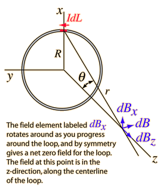
Set up coordinates with the loop in the $yz$-plane, centred at the origin, of radius $R$ carrying current $I$. The axis of the loop is the $x$-axis. We want the magnetic field at point P on the axis at distance $x$ from the centre O.

Pick a small element $d\vec{l}$ on the loop. The vector from this element to P has magnitude

$$r = \sqrt{R^2 + x^2}$$

Recall in the Biot–Savart law, the angle $\theta$ is between $d\vec{l}$ and $\vec{r}$. Here, $d\vec{l}$ is tangent to the loop (in the $yz$-plane), and the vector from the element to P points radially toward P, so $d\vec{l}\perp\vec{r}$. Hence $\sin\theta = 1$ for every element on the loop, which greatly simplifies the integral.

Applying the Biot–Savart Law

By Biot–Savart, with $\sin\theta = 1$:

$$dB = \dfrac{\mu_0}{4\pi} \dfrac{I\,dl}{r^2} = \dfrac{\mu_0 I\,dl}{4\pi\,(R^2 + x^2)}\,.$$

Next, only the axial component of $d\vec{B}$ survives after summing around the loop. Let $\phi$ be the angle between $\vec{r}$ and the $x$-axis, so

• $\cos\phi = \dfrac{x}{r}$,
• $\sin\phi = \dfrac{R}{r}$.

Since $d\vec{B}$ is perpendicular to $\vec{r}$, the angle between $d\vec{B}$ and the axis is $90^\circ - \phi$, and thus

$$dB_{\rm axis} = dB\cos(90^\circ - \phi) = dB\sin\phi = \dfrac{\mu_0 I\,dl}{4\pi\,(R^2 + x^2)} \cdot \dfrac{R}{r} = \dfrac{\mu_0 I R}{4\pi\,(R^2+x^2)^{3/2}}\,dl\,.$$

Now integrate around the loop. Since $\oint dl = 2\pi R$, we get

$$\boxed{B_{\rm axis} = \dfrac{\mu_0 I R^2}{2\,(R^2+x^2)^{3/2}}}\,.$$

For $N$ turns (a flat coil), multiply by $N$:

$$B_{\rm axis} = \dfrac{\mu_0 N I R^2}{2\,(R^2+x^2)^{3/2}}\,.$$

Direction: by the right-hand rule (thumb along $+x$ if fingers curl in current direction).

Three Special Cases You Must Know

Case 1 — Field at the centre of the loop ($x = 0$)

$$B_{\rm centre} = \dfrac{\mu_0 I R^2}{2\,(R^2 + 0)^{3/2}} = \boxed{\;\dfrac{\mu_0 I}{2R}\;}$$

For $N$ turns:

$$B_{\rm centre} = \dfrac{\mu_0 N I}{2R}\,.$$

Direction: perpendicular to the plane of the loop, by right-hand rule.

Case 2 — Field far on the axis ($x \gg R$)

When $x \gg R$, $(R^2 + x^2)^{3/2} \approx x^3$, so

$$B_{\rm axis} \approx \dfrac{\mu_0 N I R^2}{2x^3} = \dfrac{\mu_0}{4\pi}\,\dfrac{2\,m}{x^3}$$

where $$m = N I A = N I (\pi R^2)$$ is the magnetic dipole moment of the loop.

Case 3 — Half-field point ($B_{\rm axis} = B_{\rm centre}/2$)

Set

$$\dfrac{R^2}{(R^2 + x^2)^{3/2}} = \dfrac{1}{2R} \quad\Rightarrow\quad x = R\sqrt{2^{2/3}-1} \approx 0.766\,R\,.$$

Field Direction and Geometry of Lines

Right-hand rule for the loop

• Curl the fingers of the right hand in the direction of the current flow around the loop. The thumb then points in the direction of $\vec{B}$ along the axis.
• Equivalently, the face where current appears anti-clockwise is the north pole, and the clockwise face is the south pole.

Sketching the field lines

• They pass through the centre along the axis (nearly uniform locally).
• They emerge from the north face, loop around through space, and re-enter at the south face.
• Far away, they resemble a tiny bar magnet — the magnetic dipole analogy.

On-axis vs off-axis

The formula

$$B_{\rm axis} = \dfrac{\mu_0 N I R^2}{2\,(R^2+x^2)^{3/2}}$$

applies only on the axis. Off-axis fields require more involved integration.

Memory Capsule

Master formula

For a circular coil of $N$ turns, radius $R$, current $I$, on-axis distance $x$: $$B_{\rm axis} = \dfrac{\mu_0 N I R^2}{2\,(R^2 + x^2)^{3/2}}$$

Three key special cases

Location	Formula	Comment
Centre ($x = 0$)	$B_{\rm axis} = \dfrac{\mu_0 N I}{2R}$	Standard recall fact
Far on axis ($x\gg R$)	$B \approx \dfrac{\mu_0}{4\pi}\dfrac{2m}{x^3}$	$m = NI\pi R^2$, magnetic dipole field
Half-field point	$x \approx 0.766\,R$	Field drops to half at $\sim0.77R$

Right-hand rule

• Fingers curl in current direction $\Rightarrow$ thumb points along $\vec{B}_{\rm axis}$.
• Anti-clockwise face viewed $\Rightarrow$ north pole.

Dipole moment $$m = NIA = NI\pi R^2\,.$$

Solved Examples

Example 1: Field at the centre of a single loop

A circular loop of radius $5$ cm carries $2$ A. Find the magnetic field at the centre.

Solution. Use $$B = \dfrac{\mu_0 I}{2R} = \dfrac{4\pi\times10^{-7}\times2}{2\times0.05} = \dfrac{8\pi\times10^{-7}}{0.1} = 8\pi\times10^{-6}~\mathrm{T} \approx 2.51\times10^{-5}~\mathrm{T}\,.$$

Example 2: Field at the centre of a 100-turn coil

A circular coil of 100 turns has radius $10$ cm and carries $0.5$ A. Find $B$ at the centre.

Solution. $$B = \dfrac{\mu_0 N I}{2R} = \dfrac{4\pi\times10^{-7}\times100\times0.5}{2\times0.10} = \dfrac{2\pi\times10^{-5}}{0.20} = \pi\times10^{-4}~\mathrm{T} \approx 3.14\times10^{-4}~\mathrm{T}\,.$$

Example 3: Field at a point on the axis

A loop of radius $R=4$ cm carries $I=6$ A. Find $B$ on its axis at $x=3$ cm.

Solution.

1. Convert to SI: $R=0.04$ m, $x=0.03$ m.
2. Compute denominator: $$R^2+x^2 = 0.04^2 + 0.03^2 = 0.0025~\mathrm{m}^2, \quad (R^2+x^2)^{3/2} = (0.0025)^{1.5} = 0.000125~\mathrm{m}^3.$$
3. Numerator: $$\mu_0 I R^2 = (4\pi\times10^{-7})(6)(0.04^2) = (4\pi\times10^{-7})(6)(0.0016) = 3.84\pi\times10^{-9}~\mathrm{T\cdot m}^2.$$
4. Formula with the factor of 2: $$B = \dfrac{3.84\pi\times10^{-9}}{2 \times 1.25\times10^{-4}} = \dfrac{3.84\pi}{2.5}\times10^{-5} \approx 1.536\pi\times10^{-5} \approx 4.83\times10^{-5}~\mathrm{T}.$$

Example 4: Comparing centre and axial point

For the loop in Example 3, find $B_{\rm axis}(x=3\rm cm)/B_{\rm centre}$.

Solution. $$\dfrac{B_{\rm axis}}{B_{\rm centre}} = \dfrac{R^2/[2(R^2+x^2)^{3/2}]}{1/[2R]} = \dfrac{R^3}{(R^2+x^2)^{3/2}} = \Bigl(\tfrac{4}{5}\Bigr)^3 = \tfrac{64}{125} = 0.512\,.$$

Example 5: Loop in a particular orientation

A coil of radius $6$ cm, $N=50$, carries $4$ A. It lies in the $xy$-plane; current is anti-clockwise as seen from $+z$. Find $\vec B$ at the origin.

Solution. $$B = \dfrac{\mu_0 N I}{2R} = \dfrac{4\pi\times10^{-7}\times50\times4}{2\times0.06} = \dfrac{8\pi\times10^{-5}}{0.12} = \dfrac{2\pi\times10^{-3}}{3} \approx 2.09\times10^{-3}~\mathrm{T}$$ Direction: thumb along $+z$. So $\vec B = 2.09\,\hat z$ mT.

Example 6: Magnetic moment and dipole-style far field

A flat coil of $N=200$, $R=5$ cm, $I=3$ A.

(a) Magnetic dipole moment: $$m = NI\pi R^2 = (200)(3)\pi(0.05)^2 = 1.5\pi~\mathrm{A\cdot m^2} \approx 4.71~\mathrm{A\cdot m^2}.$$ (b) Field at $x=0.5$ m using dipole formula ($x/R=10\gg1$): $$B \approx \dfrac{\mu_0}{4\pi} \dfrac{2m}{x^3} = 10^{-7}\dfrac{2(4.71)}{0.5^3} \approx 7.5\times10^{-6}~\mathrm{T} = 7.5~\mu\mathrm{T}.$$

Example 7: Two concentric coplanar loops (same sense)

$R_1=4$ cm, $R_2=8$ cm, both $I=5$ A.

Solution. $$B_1 = \dfrac{\mu_0 I}{2R_1} = 5\pi\times10^{-5}~\mathrm{T}, \quad B_2 = \dfrac{\mu_0 I}{2R_2} = 2.5\pi\times10^{-5}~\mathrm{T},$$ Same direction $\Rightarrow B_{\rm net}=(5+2.5)\pi\times10^{-5}=7.5\pi\times10^{-5}\approx2.36\times10^{-4}$ T.

Example 8: Two concentric coplanar loops (opposite sense)

$R_1=5$ cm with $I_1=2$ A, $R_2=10$ cm with $I_2=4$ A, opposite sense.

Solution. $$B_1 = 8\pi\times10^{-6}~\mathrm{T}, \quad B_2 = 8\pi\times10^{-6}~\mathrm{T},$$ Opposite $\Rightarrow B_{\rm net}=0$.