We have, up to now, looked at how magnetic fields push on moving charges and current-carrying wires. Now we flip the question: given a current, what magnetic field does it produce? The fundamental answer was supplied in 1820 by two French physicists, Jean-Baptiste Biot and Félix Savart.
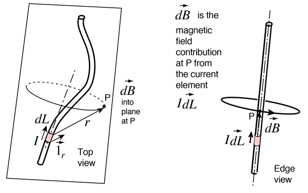
Consider a steady current I flowing through a wire. Take a tiny element dl of the wire. Let r be the position vector drawn from the element to a field point P, of magnitude r and unit vector r^. Then the magnetic field contributed by this element at P is:
dB=4πμ0r2Idl×r^
Here μ0=4π×10−7T·m/A is the permeability of free space.
Analogy with Coulomb's Law
Coulomb's law
Biot-Savart law
dE=4πε01r2dqr^
dB=4πμ0r2Idl×r^
Source: charge element dq
Source: current element Idl
Field along r^ (radial)
Field perpendicular to plane of dl and r^
∝1/r2
∝1/r2
Direction, Magnitude and Units of dB
Direction — perpendicular to the dl–r^ plane
Because dB involves dl×r^, it is perpendicular to bothdl and r^. Use the right-hand rule:
Point the fingers of your right hand along dl; curl them toward r^. Your thumb gives the direction of dB.
Magnitude
Writing ∣dl×r^∣=dlsinθ where θ is the angle between dl and r^:
dB=4πμ0r2Idlsinθ
θ=0∘ or 180∘ (on the wire's axis): dB=0.
θ=90∘ (point perpendicular to dl): dB is maximum.
Doubling I doubles dB; doubling r quarters dB.
Units
μ0 has units T·m/A. Thus μ0I/(4πr2) has units T/m, and multiplying by dl (m) gives dB in tesla.
The total field at P is obtained by integration over the entire circuit:
B(P)=4πμ0I∮r2dl×r^.
When all current elements contribute dB in the same direction—for example, points on the axis of a circular loop or any external point around a straight wire—the Biot-Savart integral reduces to a simple scalar sum.
Application 1 — Magnetic Field Due to an Infinite Straight Wire
Place an infinitely long straight wire along the y-axis, carrying current I upward. We want B at a point P at perpendicular distance d from the wire.
Choose a current element at position y: dl=dyy^.
The vector from this element to P has length r=d2+y2 and sinθ=d/r.
Every dB points into or out of the page at P (same sense everywhere), so we integrate magnitudes:
dB=4πμ0Ir2dysinθ=4πμ0I(d2+y2)3/2ddy.
Integrate y from −∞ to +∞:
B=4πμ0Id∫−∞∞(d2+y2)3/2dy=2πdμ0I.
Result:
B=2πdμ0I
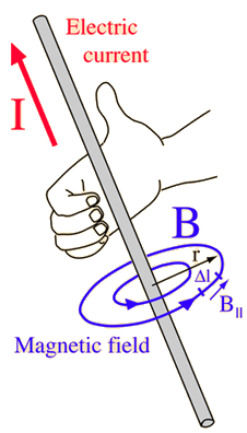
Geometry of field lines: concentric circles around the wire; sense by right-hand thumb rule.
Note the 1/d fall-off arises from integrating an inverse-square element over an infinite line.
Application 2 — Magnetic Field Due to a Finite Straight Wire
For a straight segment of current I, drop a perpendicular from P to the wire at foot F; let d=PF. Draw lines from P to the segment ends, making angles α1, α2from the perpendicular. A direct integration gives:
B=4πdμ0I(sinα1+sinα2)
Direction: perpendicular to the plane of the wire and P, by the right-hand rule.
Special cases:
Infinite wire: α1=α2=90∘⇒B=μ0I/(2πd).
Semi-infinite wire: one angle 0∘, the other 90∘, gives B=μ0I/(4πd).
When solving finite-wire problems, sketch the geometry first. Mark angles from the perpendicular, using negative signs if P lies off one end (so that sin(−α)=−sinα).
Memory Capsule
Biot-Savart law (memorise):dB=4πμ0r2Idl×r^,μ0=4π×10−7T⋅m/A
A long straight wire carries current 5A. Find the magnetic field at a point 10cm from the wire.
Solution. Use B=μ0I/(2πd) with I=5A, d=0.10m.
Since μ0/(2π)=2×10−7T·m/A,
B=0.102×10−7×5=1×10⁻⁵T=10μT.
Example 2: Doubling the current, doubling the distance
A long straight wire produces a field of 4×10⁻⁵T at 5cm. What is the field at 10cm if the current is doubled?
Solution.B∝I/d. Bnew=4×10−5×22=4×10⁻⁵T.
Example 3: Field due to a current element
A current element Idl=2×10⁻⁴x^ A·m is at the origin. Find dB at (0,0.5,0) m.
Solution.r=0.5y^, so r^=y^, r=0.5 m. dB=4πμ0r2Idl×r^=(10−7)0.252×10⁻⁴(x^×y^)=8×10⁻¹¹z^T.
Example 4: Two parallel wires, field at midpoint
Two long parallel wires carry I1=6A and I2=4A in the same direction, separated by 20cm. Find B at the midpoint.
Solution. Each wire at distance 0.10m: B1=2π(0.10)μ0I1=1.2×10⁻⁵T,B2=0.8×10⁻⁵T.
The fields oppose, so Bnet=∣B1−B2∣=4×10⁻⁶T, toward the weaker wire.
Example 5: Field due to a finite wire — symmetric case
A wire of length 2L=20cm carries I=10A. Find B at a point 10cm from its centre.
Solution.L=d=0.10 m, so sinα=L/L2+d2=1/2. B=4πdμ0I(2sinα)=(10−7)0.101022=10−52T≈14.1μT.
Example 6: Semi-infinite wire
A wire extends from the origin to +∞ on the x-axis, carrying I=8A. Find B at (0,5cm,0).
Solution. Semi-infinite: one angle 0∘, one 90∘. B=4πdμ0I=(10−7)0.058=1.6×10⁻⁵T.
Example 7: Anti-parallel currents
Two long parallel wires, 4cm apart, carry 5A in opposite directions. Find B at a point 1cm from one wire and 5cm from the other.
Solution.B1=1.0×10⁻⁴T at 0.01 m, B2=2.0×10⁻⁵T at 0.05 m.
Outside the gap, they subtract: Bnet=1.0×10⁻⁴−2.0×10−5=8.0×10⁻⁵T.
Example 8: Recovering Coulomb-style 1/r2
A short element Idl=1mm at I=1 A produces dB at r=0.10m. Compare with the electric field of q=1nC at the same r.
Solution.
Magnetic: dB=10−70.0110−3=10−8T.
Electric: E=9×1090.0110−9=900V/m.
Both fall as 1/r2, but magnetic fields from small currents are much weaker.
Ready to test your knowledge?
Take a quick interactive quiz on this topic —
free, works without login.