JEE Corner — Advanced Thermal Physics

What JEE Adds to This Chapter

Sections 1 to 12 built this chapter properly. Expansion, specific heat, calorimetry, latent heat, conduction, convection, radiation and cooling are all in place, and for the Board paper that build is complete.

What JEE adds is not new physics. It is still $\Delta L = \alpha L \Delta T$, still $Q = ms\Delta T$, still $H = \frac{KA\Delta T}{L}$, still $\sigma A e T^4$. What changes is that the quantity you want stops being uniform.

The rod is no longer the same thickness at both ends. The conductivity is no longer the same at both ends. The heat no longer flows through a fixed area, because the area is a shell that grows as you move outward. The ice sheet that is conducting the heat is itself getting thicker while you watch. The mixture's final state is not given to you — you have to work out whether the ice all melted before you can even write the balance.

Every one of those is answered the same way: stop assuming the thing is constant, take a slice, and add the slices up. And before you write a single temperature into a fourth power, say out loud whether it is in kelvin.

Some of what follows sits outside the rationalised syllabus body text — thermal resistance and series-parallel networks, bimetallic strips, Kirchhoff's law — but JEE Main and JEE Advanced ask this material every year, so it is developed here from first principles.

The eleven things this section teaches

#	Skill	Why it earns marks
1	A composite rod's effective $\alpha$, and the condition for the difference of two lengths to stay constant	One line of algebra, asked as a full question
2	The pendulum clock — the temperature for correct time, and the seconds gained or lost per day	The only place a $\frac{1}{2}$ from a binomial expansion earns four marks
3	Apparent versus real expansion, and the weight thermometer	Two coefficients that differ by the vessel's, and a mass that gets expelled
4	The bimetallic strip's radius of curvature	Pure geometry once you see that both mid-lines turn through the same angle
5	Conduction through a rod of varying cross-section, by integration	The answer is a geometric mean, and the guess is always wrong
6	Conduction with $K$ varying along the length	Resistances in series, taken to the continuum limit
7	Radial conduction through pipe lagging and through a spherical shell	Needs $\int \frac{dr}{r}$; a slab formula is not merely inaccurate, it is meaningless
8	Growth of ice on a pond and the time to thicken from one depth to another	The famous $t \propto y^2$
9	Networks with junction temperatures, series, parallel and star	Equal heat current at every node is the whole method
10	Multi-phase calorimetry where the final state must be determined	Assume it and you will be wrong roughly half the time
11	Radiation exchange, equilibrium in sunlight, and Newton's law in exponential form	Fourth powers, kelvin, and knowing where the linear law dies

Conventions, fixed now

This section uses the chapter's symbol table without exception. Restating the five that matter here:

• $T$ is an absolute temperature in kelvin. $t$ or $t_C$ is Celsius. Every fourth power, every ratio, every gas-law step needs kelvin.
• $L$ bare is a length; $L_f$ and $L_v$ are the latent heats of fusion and vaporisation.
• $\alpha$ is linear expansion, $\beta$ areal, $\gamma$ volume. Absorptive power is $a$, never $\alpha$.
• $K$ is thermal conductivity; lowercase $k$ is the cooling constant in Newton's law.
• $s$ is specific heat capacity, $C$ molar specific heat, $S$ the heat capacity of a whole body. $R$ is thermal resistance $\frac{L}{KA}$, in K/W. The one exception is the solar constant, also written $S$, in W/m$^2$ — the units separate them wherever both appear.

Constants used throughout, unless a problem states otherwise:

Quantity	Value
$\alpha_{\text{steel}}$	$1.2 \times 10^{-5}$ K$^{-1}$
$\alpha_{\text{brass}}$	$1.8 \times 10^{-5}$ K$^{-1}$
$\alpha_{\text{copper}}$	$1.7 \times 10^{-5}$ K$^{-1}$
$\gamma_{\text{mercury}}$	$1.82 \times 10^{-4}$ K$^{-1}$
$s_{\text{water}}$	4186 J/(kg K)
$s_{\text{ice}}$	2100 J/(kg K)
$L_f$ (ice)	$3.33 \times 10^{5}$ J/kg
$L_v$ (water)	$22.6 \times 10^{5}$ J/kg
$K_{\text{copper}}$	385 W/(m K)
$K_{\text{steel}}$	50.2 W/(m K)
$K_{\text{ice}}$	1.6 W/(m K)
$\sigma$	$5.67 \times 10^{-8}$ W/(m$^2$ K$^4$)
Density of ice	900 kg/m$^3$

Every solution restates the constants it uses. No problem here mixes two values of the same constant.

Key Point — the master move of this whole section: $$R_{th} = \int \frac{dx}{K(x)\,A(x)} \qquad\text{and}\qquad H = \frac{\Delta T}{R_{th}}$$ Thermal resistance is what adds. Take a slab so thin that $K$ and $A$ are constant across it, write its resistance, and integrate along the path the heat takes. Every non-uniform conduction problem in this section is that one integral with a different $A(x)$. For a slab $A$ is constant; for a taper $A = \pi r(x)^2$; for a pipe $A = 2\pi r L$; for a sphere $A = 4\pi r^2$.

[Exam Tip] Three questions, asked before any algebra, choose the method for almost every problem below. Is the cross-section the same everywhere? Is the conductivity the same everywhere? Is anything changing while the heat flows? A "no" to the first two means integrate. A "no" to the third means write a differential equation in time. Answer all three and you have chosen your method before writing a symbol.

Composite Rods, the Frozen Gap, and the Pendulum Clock

A rod made of two metals

Join a rod of length $L_1$ and coefficient $\alpha_1$ end to end with a rod of length $L_2$ and coefficient $\alpha_2$. Heat the pair through $\Delta T$. Each piece expands on its own account, so the total elongation is

$$\Delta L = L_1\alpha_1\Delta T + L_2\alpha_2\Delta T$$

Define the effective coefficient of the composite by insisting it behaves like a single rod of length $L_1 + L_2$:

Key Point — effective linear expansion coefficient: $$\alpha_{\text{eff}} = \frac{L_1\alpha_1 + L_2\alpha_2}{L_1 + L_2}$$ It is the length-weighted average of the two coefficients, not the plain average. The longer piece gets more of a say.

Note carefully what this is not. It is not $\frac{\alpha_1+\alpha_2}{2}$ unless the two lengths happen to be equal. And it is not the parallel-resistor-looking $\frac{2\alpha_1\alpha_2}{\alpha_1+\alpha_2}$ — that formula belongs to a different problem (two rods side by side with a common expansion), and mixing them up is a standard way to lose four marks.

The difference that refuses to change

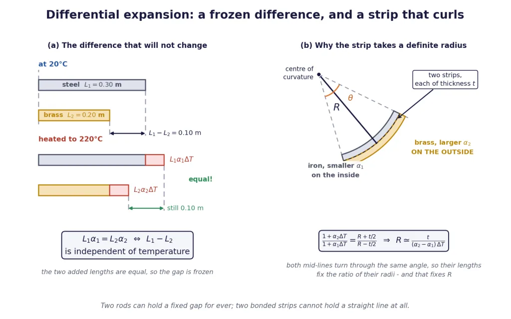
Here is the classic. Two rods of different metals are laid side by side, not joined. We want the difference in their lengths to be the same at every temperature. What does that demand?

At temperature $t$ the two lengths are $L_1(1+\alpha_1\Delta T)$ and $L_2(1+\alpha_2\Delta T)$, so the difference is

$$L_1 - L_2 + \left(L_1\alpha_1 - L_2\alpha_2\right)\Delta T$$

For that to be independent of $\Delta T$, the bracket must vanish.

Key Point — the frozen-gap condition: $$L_1\alpha_1 = L_2\alpha_2 \qquad\Longleftrightarrow\qquad \frac{L_1}{L_2} = \frac{\alpha_2}{\alpha_1}$$ Read it physically: the two rods must grow by the same absolute amount. Then whatever gap there was between their ends stays exactly that gap. The rod with the smaller $\alpha$ has to be the longer one, which is the part students get backwards.

That is the whole trick behind a gridiron pendulum and behind the invar-and-brass compensating strips inside a good clock: not to stop things expanding, but to arrange that two expansions cancel out where it matters.

The pendulum clock

A pendulum clock counts time by counting swings. Its period is

$$T_p = 2\pi\sqrt{\frac{L}{g}}$$

Heat the pendulum and $L$ grows, so $T_p$ grows, so each swing takes longer and the clock runs slow. Cool it and the clock runs fast.

Put in $L^{\,\prime} = L(1+\alpha\Delta T)$:

$$\frac{T_p^{\,\prime}}{T_p} = \sqrt{1+\alpha\Delta T} \approx 1 + \frac{1}{2}\alpha\Delta T$$

using the binomial expansion, which is superb here because $\alpha\Delta T$ is of order $10^{-4}$.

Key Point — the clock formula: $$\frac{\Delta T_p}{T_p} = \frac{1}{2}\alpha\,\Delta T$$ and the time gained or lost in one day of 86400 seconds is $$\left\lvert \Delta t \right\rvert = \frac{1}{2}\alpha\,\Delta T \times 86400 \ \text{s}$$ Slow if the pendulum is warmer than the calibration temperature, fast if it is cooler. The $\frac{1}{2}$ is the entire question; forget it and your answer is exactly double.

Three shapes this comes in:

1. Given the calibration temperature and the room temperature, find the daily error. Straight substitution.
2. Given the daily error, find the temperature at which the clock is correct. Solve for $\Delta T$, then add or subtract from the stated temperature — and check the sign by asking whether the clock is gaining or losing.
3. Given errors at two temperatures, find $\alpha$ or the correct temperature. The error is linear in temperature, so two points fix the line. Where the line crosses zero is where the clock is right.

[Exam Tip] The daily error per kelvin is $\frac{1}{2}\alpha \times 86400 = 43200\,\alpha$ seconds. For steel, $\alpha = 1.2\times10^{-5}$ K$^{-1}$, that is 0.518 s per day per kelvin. Memorise that one number and most clock questions become mental arithmetic: 20 K of warming costs about 10.4 s a day.

Liquids, the Weight Thermometer, and the Bimetallic Radius

Apparent expansion: you cannot see the vessel move

Heat a flask of mercury and the mercury level rises. But the flask expanded too, so the rise you actually observe is short of the true expansion of the liquid.

Let the flask hold volume $V_0$ of liquid at $0$°C. Heat both through $\Delta T$:

• the liquid wants to occupy $V_0(1+\gamma_r\Delta T)$, where $\gamma_r$ is its real coefficient of volume expansion;
• the flask now holds $V_0(1+\gamma_g\Delta T)$;
• the overflow, or the visible rise, corresponds to the difference.

Key Point — apparent expansion: $$\gamma_{\text{app}} = \gamma_{\text{real}} - \gamma_{\text{vessel}}$$ and since the vessel is a solid, $\gamma_{\text{vessel}} = 3\alpha_{\text{vessel}}$. What you measure in a flask is always $\gamma_{\text{app}}$. The real coefficient is only reachable if you know the vessel's material — or if you use a method that eliminates the vessel entirely.

Because $\gamma$ for a liquid is typically ten times $\gamma$ for glass, the correction is real but not enormous. For mercury in glass, $\gamma_r = 1.82\times10^{-4}$ K$^{-1}$ and $\gamma_g = 2.7\times10^{-5}$ K$^{-1}$, so $\gamma_{\text{app}} = 1.55\times10^{-4}$ K$^{-1}$ — about 15% below the real value. Quote the wrong one and you are 15% out.

The weight thermometer

Now the beautiful version. Fill a bulb completely with liquid at $t_1$, seal nothing, heat it to $t_2$ and catch what spills out. Weigh the spilt liquid. That is a weight thermometer, and it is how $\gamma_{\text{app}}$ is actually measured.

Take $t_1 = 0$°C so that the mass in the bulb is $m$ and the liquid's density there is $\rho_0$. At temperature $t$:

• the volume that overflows is $V_0\,\gamma_{\text{app}}\,t$, measured at the hot temperature;
• the density of the hot liquid is $\rho_t = \dfrac{\rho_0}{1+\gamma_r t}$.

Multiply:

Key Point — mass expelled by a weight thermometer: $$m^{\,\prime} = \frac{m\,\gamma_{\text{app}}\,t}{1+\gamma_r\,t}$$ The denominator is there because the expelled liquid is hot, therefore less dense, so the same volume weighs less. It is often dropped, giving $m^{\,\prime} = m\gamma_{\text{app}}t$; that is a fine first estimate but it runs about $\gamma_r t$ high — for mercury over 100 K, about 1.8% high.

Rearranged for the experimenter:

$$\gamma_{\text{app}} \approx \frac{m^{\,\prime}}{\left(m - m^{\,\prime}\right)t}$$

which is the form to use when the question gives you the mass remaining rather than the mass expelled. But notice the $\approx$: only the first form is exact. Put $m^{\,\prime} = \frac{m\gamma_{\text{app}}t}{1+\gamma_r t}$ into it, so that the mass left behind is $m - m^{\,\prime} = \frac{m\left(1+\gamma_g t\right)}{1+\gamma_r t}$, and the $\gamma_r$ cancels to leave

$$\frac{m^{\,\prime}}{\left(m - m^{\,\prime}\right)t} = \frac{\gamma_{\text{app}}}{1+\gamma_g\,t}$$

So the remaining-mass form returns $\gamma_{\text{app}}$ low by the factor $1+\gamma_g t$ — the vessel's own expansion, which this rearrangement cannot see. For mercury in glass over 100 K that factor is $\gamma_g t = 2.7\times10^{-3}$, so the answer comes out about 0.3% low: harmless in an exam, but it is an approximation and not an identity. Multiply by $\left(1+\gamma_g t\right)$ if you ever need it exact.

The bimetallic strip, and its radius of curvature

Bond a strip of brass to a strip of iron, both of the same length at room temperature. Heat them. Brass wants to be longer than iron does, they are stuck together, so the only way both can be satisfied is for the pair to bend, with the brass on the outside where the arc is longer.

Take each strip to have thickness $t$, so the pair has total thickness $2t$. After heating through $\Delta T$ the strip becomes an arc of radius $R$, measured to the bonded interface, subtending an angle $\theta$ at the centre.

The key observation: both mid-lines turn through the same angle $\theta$. They are stuck together, so they must. The mid-line of the inner strip sits at radius $R - \frac{t}{2}$ and the mid-line of the outer at $R + \frac{t}{2}$, and each has the length free expansion would have given it:

$$L\left(1+\alpha_1\Delta T\right) = \left(R - \tfrac{t}{2}\right)\theta, \qquad L\left(1+\alpha_2\Delta T\right) = \left(R + \tfrac{t}{2}\right)\theta$$

Divide one by the other and the unknowns $L$ and $\theta$ both disappear:

$$\frac{1+\alpha_2\Delta T}{1+\alpha_1\Delta T} = \frac{R+\frac{t}{2}}{R-\frac{t}{2}}$$

Apply componendo and dividendo — subtract the two sides' numerators and denominators, then add them:

$$\frac{\left(\alpha_2-\alpha_1\right)\Delta T}{2+\left(\alpha_1+\alpha_2\right)\Delta T} = \frac{t}{2R}$$

Key Point — radius of curvature of a bimetallic strip: $$R = \frac{t\left[\,2+\left(\alpha_1+\alpha_2\right)\Delta T\,\right]}{2\left(\alpha_2-\alpha_1\right)\Delta T} \;\approx\; \frac{t}{\left(\alpha_2-\alpha_1\right)\Delta T}$$ with $t$ the thickness of EACH strip, so $2t$ is the thickness of the pair. The same result is often written using the total thickness $d = 2t$, giving $R \approx \frac{d}{2(\alpha_2-\alpha_1)\Delta T}$ — identical physics, so read which thickness a formula means before you use it. The dropped term is of order $\left(\alpha_1+\alpha_2\right)\Delta T \sim 10^{-3}$, so the approximation is good to about a tenth of a percent.

Three things to read off that result, because each is a question in its own right:

• $R \propto \frac{1}{\Delta T}$. Double the heating, halve the radius, so the strip curls twice as tightly. That is exactly what makes it a usable thermostat: the deflection is proportional to temperature.
• $R \propto t$. A thinner pair curls more. Thermostat strips are thin for that reason, not to save metal.
• $R$ depends only on the difference of the coefficients. Two metals with $\alpha$ values of $1.2\times10^{-5}$ and $1.8\times10^{-5}$ behave exactly like a pair with $2.2\times10^{-5}$ and $2.8\times10^{-5}$.

For a strip of length $L$ clamped at one end, the free tip swings sideways through

$$\delta = R\left(1 - \cos\frac{L}{R}\right) \;\approx\; \frac{L^{2}}{2R}$$

[Exam Tip] Which way does it bend? Say it in words rather than trusting a formula: on heating it bends towards the metal that expands less; on cooling it bends towards the metal that expands more. Iron-brass heated curls with brass outside; the same strip cooled below its flat temperature curls the other way, with iron outside.

Conduction When the Rod Is Not Uniform

Everything in Section 8 assumed a bar of constant cross-section made of one material, and gave $H = \frac{KA\Delta T}{L}$. Take away either assumption and that formula is not merely inaccurate — it does not have a well-defined $A$ or $K$ to put into it.

The fix is the same one every time. Resistances in series add, so slice the rod into slabs so thin that $K$ and $A$ are constant across each, and integrate.

$$R_{th} = \int_0^{L}\frac{dx}{K(x)\,A(x)}, \qquad H = \frac{\Delta T}{R_{th}}$$

Two facts make this workable, and both are worth saying out loud before you start:

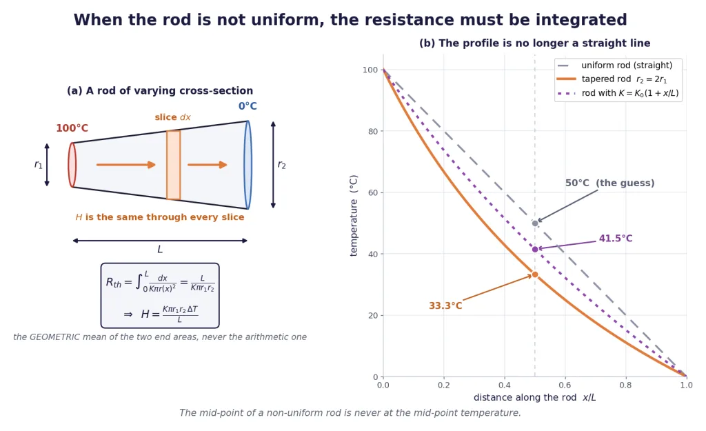
1. In the steady state, $H$ is the same through every slice. Nothing is accumulating anywhere, so whatever enters a slice must leave it. This is what lets you treat $H$ as a constant and pull it out of the integral.
2. The temperature gradient is therefore steepest where $KA$ is smallest. The heat has to squeeze through, and it needs a bigger push to do it. That single sentence predicts the shape of every profile below before you integrate anything.

A rod of varying cross-section: the truncated cone

A solid rod tapers uniformly from radius $r_1$ at the hot end to $r_2$ at the cold end over a length $L$, and its conductivity $K$ is uniform. At distance $x$,

$$r(x) = r_1 + \frac{\left(r_2-r_1\right)x}{L}, \qquad A(x) = \pi r(x)^2$$

$$R_{th} = \int_0^{L}\frac{dx}{K\pi r(x)^2} = \frac{L}{K\pi\left(r_2-r_1\right)}\left[\frac{1}{r_1}-\frac{1}{r_2}\right] = \frac{L}{K\pi r_1 r_2}$$

Key Point — the tapered rod: $$H = \frac{K\pi r_1 r_2\,\Delta T}{L}$$ The effective area is $\pi r_1 r_2$ — the geometric mean of the two end areas, $\sqrt{A_1A_2}$. It is not the arithmetic mean $\frac{A_1+A_2}{2}$, and it is not the area at the mid-point. Put $r_1 = r_2 = r$ and it collapses correctly to $\frac{K\pi r^2\Delta T}{L}$, which is your check that the algebra is right.

And the temperature at a point is not what you would guess. The profile follows from integrating only as far as $x$:

$$T(x) = T_1 - \frac{H}{K\pi}\cdot\frac{L}{r_2-r_1}\left[\frac{1}{r_1}-\frac{1}{r(x)}\right]$$

For a rod running from 100°C to 0°C with $r_2 = 2r_1$, the mid-point sits at 33.3°C, not 50°C. It is bunched toward the cold end because the thin half has most of the resistance, so most of the temperature drop happens there. Draw the profile once and you will never guess 50 again.

A rod whose conductivity varies along its length

Now keep the area constant and let the material change, say $K(x) = K_0\left(1+\frac{x}{L}\right)$: conductivity $K_0$ at the hot end rising to $2K_0$ at the cold end.

$$R_{th} = \int_0^{L}\frac{dx}{K_0\left(1+\frac{x}{L}\right)A} = \frac{L}{K_0A}\ln 2$$

$$H = \frac{K_0A\,\Delta T}{L\ln 2} = \frac{K_0 A \Delta T}{0.693\,L}$$

so the equivalent conductivity of the whole rod is

$$K_{\text{eq}} = \frac{K_0}{\ln 2} = 1.443\,K_0$$

Key Point: The rod behaves as though its conductivity were $1.443\,K_0$, not the arithmetic mean $1.5\,K_0$ of its end values. The equivalent conductivity of a series arrangement is always dragged below the arithmetic mean, because the poor conductor is the bottleneck and bottlenecks dominate series resistance.

The temperature profile is logarithmic here: $T(x) = T_1 - \frac{\Delta T\,\ln\left(1+\frac{x}{L}\right)}{\ln 2}$, which for 100°C to 0°C puts the mid-point at 41.5°C. Again below 50, and for the same reason — the resistive half is nearer the hot end.

The two profiles side by side

Rod	$H$	Mid-point temperature for 100°C to 0°C
uniform, area $A$, conductivity $K$	$\dfrac{KA\Delta T}{L}$	50.0°C
tapered, $r_2 = 2r_1$	$\dfrac{K\pi r_1r_2\Delta T}{L}$	33.3°C
$K = K_0\left(1+\frac{x}{L}\right)$	$\dfrac{K_0A\Delta T}{L\ln 2}$	41.5°C

[Exam Tip] Two checks worth five seconds each. First, set the varying quantity constant and see whether your formula collapses to $\frac{KA\Delta T}{L}$. If it does not, the integration is wrong. Second, ask which half has the greater resistance and check that most of the temperature drop happened there. A profile that drops more across the fat, well-conducting half is telling you the integral was set up backwards.

Radial Conduction: Pipes and Shells

Lag a steam pipe. Heat leaves the pipe and travels outward through the lagging. What area is it crossing?

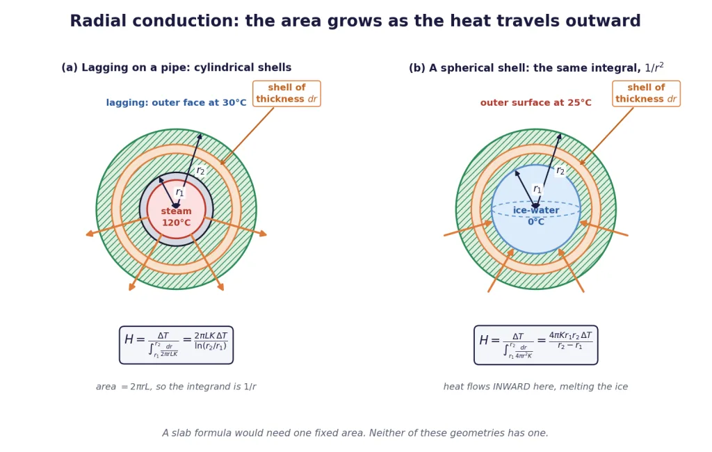
There is no single answer — that is the whole point. Just outside the pipe the heat crosses a small cylinder; at the outer surface of the lagging it crosses a much larger one. A slab formula needs one fixed area, and this geometry does not have one. So we slice again, this time into shells.

Cylindrical lagging

Take a shell of radius $r$ and thickness $dr$, on a pipe of length $L$. Its area is $2\pi r L$ and its resistance is

$$dR = \frac{dr}{K\left(2\pi r L\right)}$$

In the steady state the same $H$ crosses every shell, so the resistances are in series and simply add:

$$R_{th} = \int_{r_1}^{r_2}\frac{dr}{2\pi r L K} = \frac{1}{2\pi L K}\ln\frac{r_2}{r_1}$$

Key Point — radial conduction through a cylindrical shell: $$H = \frac{2\pi L K\left(T_1 - T_2\right)}{\ln\left(\frac{r_2}{r_1}\right)}$$ The logarithm is the signature of cylindrical geometry, and it comes from $\int\frac{dr}{r}$ and nowhere else. The temperature at any intermediate radius is $$T(r) = T_1 - \left(T_1-T_2\right)\frac{\ln\left(\frac{r}{r_1}\right)}{\ln\left(\frac{r_2}{r_1}\right)}$$

Read that profile carefully, because it contains a trap. Halfway in radius is not halfway in temperature. For lagging running from 5.0 cm to 10.0 cm with faces at 120°C and 30°C, the radius 7.5 cm sits at 67.4°C, not 75°C. Most of the temperature drop happens in the inner shells, where the area is small and the resistance per unit thickness is large.

The doubling trap. Because the answer depends on $\ln\frac{r_2}{r_1}$, doubling the thickness of the lagging does not halve the loss. Going from $r_2 = 2r_1$ to $r_2 = 3r_1$ changes the heat loss by a factor $\frac{\ln 2}{\ln 3} = 0.631$ — a 37% saving for a doubling of the lagging material. Insulation has diminishing returns, and the logarithm is why.

The spherical shell

Same method, different area law. A shell at radius $r$ has area $4\pi r^2$:

$$R_{th} = \int_{r_1}^{r_2}\frac{dr}{4\pi r^{2}K} = \frac{1}{4\pi K}\left[\frac{1}{r_1}-\frac{1}{r_2}\right] = \frac{r_2-r_1}{4\pi K r_1 r_2}$$

Key Point — radial conduction through a spherical shell: $$H = \frac{4\pi K r_1 r_2\left(T_1-T_2\right)}{r_2-r_1}$$ Here the effective area is $4\pi r_1 r_2$ — the geometric mean of the inner and outer surface areas, exactly as it was for the tapered rod, and for exactly the same reason: the integrand went as $\frac{1}{r^2}$. The profile is $T(r) = T_1 - \left(T_1-T_2\right)\dfrac{\frac{1}{r_1}-\frac{1}{r}}{\frac{1}{r_1}-\frac{1}{r_2}}$.

The family, in one table

Geometry	Area crossed	Resistance	Effective area
slab, thickness $L$	$A$, constant	$\dfrac{L}{KA}$	$A$
tapered rod, radii $r_1$, $r_2$	$\pi r(x)^2$	$\dfrac{L}{K\pi r_1r_2}$	$\pi r_1 r_2$
cylindrical shell, length $L$	$2\pi rL$	$\dfrac{\ln\left(\frac{r_2}{r_1}\right)}{2\pi LK}$	logarithmic mean
spherical shell	$4\pi r^2$	$\dfrac{r_2-r_1}{4\pi Kr_1r_2}$	$4\pi r_1 r_2$

Every row is the same integral $\int \frac{dr}{KA(r)}$ with a different $A(r)$.

[Exam Tip] How to tell instantly which one you are in. If the two faces are flat and parallel, it is a slab. If they are two circles of different radii about a common axis, it is cylindrical and you will get a logarithm. If they are two spheres about a common centre, you will get $\frac{1}{r_1}-\frac{1}{r_2}$. Getting a logarithm out of a spherical problem, or a $\frac{1}{r}$ difference out of a cylindrical one, is a sign you integrated the wrong area law — check before you substitute numbers.

Networks, Junction Temperatures, and the Growing Ice Sheet

The whole method for a network, in one sentence

In the steady state the heat current into every junction equals the heat current out of it. That is it. Write that equation at each junction and you have as many equations as unknown junction temperatures.

It is worth naming what this is: an exact analogue of Kirchhoff's current law, with $\Delta T$ playing the part of voltage, $H$ the part of current, and $R = \frac{L}{KA}$ the part of resistance. Series resistances add; parallel ones combine as reciprocals. In a JEE question you will almost always be faster writing thermal resistances than quoting an equivalent-conductivity formula, because the resistance route never asks you to remember whether the rods were in series or in parallel — the circuit tells you.

Two rods in series, and where the junction sits

Two rods of the same cross-section $A$ and length $L$, conductivities $K_1$ and $K_2$, joined end to end, free ends held at $T_1$ and $T_2$. Equal current through both:

$$\frac{T_1 - T_j}{R_1} = \frac{T_j - T_2}{R_2} \qquad\Longrightarrow\qquad T_j = \frac{\frac{T_1}{R_1} + \frac{T_2}{R_2}}{\frac{1}{R_1}+\frac{1}{R_2}} = \frac{K_1T_1 + K_2T_2}{K_1+K_2}$$

(the last step only when the two rods share $L$ and $A$).

Key Point: The junction temperature is a conductance-weighted average of the two end temperatures. The better conductor pulls the junction toward its own end. Copper against steel is 385 against 50.2, so the junction ends up within a dozen degrees of the copper end — which is exactly why a copper handle on a hot pan is a bad idea and a steel one is survivable.

And the equivalent conductivity of the pair, for equal lengths:

$$K_{\text{series}} = \frac{2K_1K_2}{K_1+K_2}, \qquad K_{\text{parallel}} = \frac{K_1+K_2}{2}$$

The first is a harmonic mean and always sits closer to the smaller conductivity; the second is an arithmetic mean and always sits in the middle. If you cannot remember which is which, rebuild them from resistances in ten seconds rather than guessing.

A star of three rods

Three rods meet at a common junction, their other ends held at $T_1$, $T_2$ and $T_3$. There is one unknown, the junction temperature $T^{\,\star}$, and one equation:

$$\frac{T_1-T^{\,\star}}{R_1} + \frac{T_2-T^{\,\star}}{R_2} + \frac{T_3-T^{\,\star}}{R_3} = 0 \qquad\Longrightarrow\qquad T^{\,\star} = \frac{\sum \frac{T_i}{R_i}}{\sum \frac{1}{R_i}}$$

Write the currents all flowing in and set the sum to zero. Then a negative answer for one of them simply means that rod is carrying heat away, and no sign has to be guessed in advance. This one habit removes most of the sign errors in network questions.

The growth of ice on a pond

Now the famous one, and the only conduction problem in this section where something is changing with time.

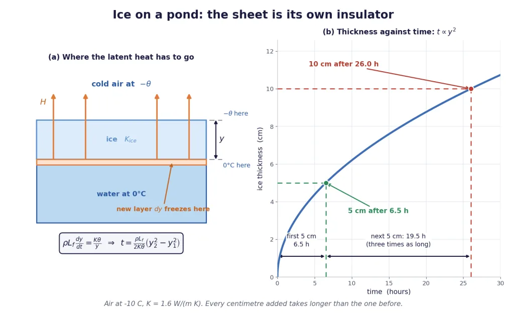
A pond has frozen to depth $y$. The air above is at $-\theta$ (with $\theta$ a positive number of degrees below zero), the water below is at 0°C, and the ice in between conducts. For a new layer of thickness $dy$ to freeze onto the underside, its latent heat must be carried up through the ice already there.

Heat released by freezing a layer $dy$ over an area $A$: $$dQ = \left(\rho A\,dy\right)L_f$$

Heat conducted up through the sheet in time $dt$, treating the sheet as a slab of thickness $y$: $$dQ = \frac{KA\theta}{y}\,dt$$

Two things deserve a moment. First, the temperature difference across the sheet is $\theta$, not $\theta$ plus anything — the underside is pinned at 0°C because that is where ice and water coexist. Second, we are treating the conduction as quasi-steady: the sheet thickens so slowly compared with how fast it reaches its steady gradient that using the steady-state formula at each instant is an excellent approximation.

Equate and separate:

$$\rho L_f\,y\,dy = K\theta\,dt \qquad\Longrightarrow\qquad \int_{y_1}^{y_2} y\,dy = \frac{K\theta}{\rho L_f}\int_0^{t}dt$$

Key Point — time for ice to thicken: $$t = \frac{\rho L_f}{2K\theta}\left(y_2^{2}-y_1^{2}\right)$$ and starting from bare water, $y_1 = 0$, this is $t = \dfrac{\rho L_f\,y^{2}}{2K\theta}$, so the thickness grows as the square root of time.

Three consequences, each of which has been an exam question:

• Going from 5 cm to 10 cm takes three times as long as going from 0 to 5 cm, because $10^2 - 5^2 = 75$ against $5^2 - 0 = 25$. The ice sheet is its own insulator, and the thicker it gets the more slowly it grows. This is why deep lakes never freeze solid.
• Doubling the thickness costs four times the total time, so a pond that froze to 10 cm in a day needs four days to reach 20 cm at the same air temperature.
• The rate at any instant is $\frac{dy}{dt} = \frac{K\theta}{\rho L_f y}$, so if a question asks how fast the ice is thickening right now, differentiate rather than dividing the total thickness by the total time.

[Exam Tip] Use the ice density, about 900 kg/m$^3$, not the water density. Some questions hand you 917 and some hand you 1000; use whatever the question states and say so in your solution. The answer scales directly with it, so a silently assumed 1000 against a stated 900 is an 11% error.

Multi-Phase Calorimetry, Radiation Exchange, and Newton's Law Honestly

When you do not know the final state

The calorimetry of Section 6 was straightforward because you were told what happened. At JEE level you are not. Mix steam with ice and any of these can be the answer:

• everything ends as water between 0°C and 100°C;
• everything pins at 0°C with ice and water coexisting;
• everything pins at 100°C with water and steam coexisting;
• rarely, it all ends as ice below 0°C.

Guessing wrong does not cost you a mark or two. It costs the whole question, because the equation you wrote was the wrong equation.

Key Point — the method that never fails: 1. Pick a reference state — 0°C water is convenient. 2. Compute the heat available from the hot side down to that reference, as a single number. 3. Compute the heat required by the cold side up to that reference, as a single number. 4. Compare them, and only then write the balance for the branch you are actually in. Do steps 2 and 3 as separate numbers on separate lines. The comparison is the physics; the arithmetic afterwards is bookkeeping.

The three tests, written out:

Compare	Conclusion
available heat $<$ heat needed to warm the ice to 0°C	final state is ice below 0°C; not all the steam condenses
heat needed to warm the ice to 0°C $<$ available $<$ that plus $m_{\text{ice}}L_f$	pins at 0°C, ice and water together; find how much ice melts
available $>$ that plus $m_{\text{ice}}L_f$	all the ice melts; solve for a final temperature above 0°C, then check it came out below 100

And check the answer against its own branch. A final temperature of 115°C from a case you assumed ended as water means the assumption was wrong, not that water reached 115°C. A final temperature outside the branch you assumed is the equation telling you to go back to step 4.

Radiation exchange and the equilibrium temperature

A body of area $A$, emissivity $e$ and absolute temperature $T$ in surroundings at $T_s$ loses net power

$$P_{\text{net}} = \sigma A e\left(T^{4} - T_s^{4}\right)$$

Key Point — the kelvin rule, in the place it matters most: $T$ and $T_s$ in that expression are absolute temperatures in kelvin, always. A body at 727°C radiates $\left(\frac{1000}{500}\right)^4 = 16$ times as much as one at 227°C. Feed the Celsius numbers in and you get $\left(\frac{727}{227}\right)^4 = 105$, which is wrong by a factor of nearly seven. Write "K" next to every temperature you substitute into a fourth power.

Equilibrium in sunlight. A body absorbing sunlight settles at the temperature where absorption balances emission. For a sphere of radius $r$ in space, sunlight of flux $S$ falls on the cross-section $\pi r^2$ but the body radiates from its whole surface $4\pi r^2$:

$$a\,S\,\pi r^{2} = e\,\sigma\left(4\pi r^{2}\right)T^{4} \qquad\Longrightarrow\qquad T = \left(\frac{a\,S}{4e\,\sigma}\right)^{1/4}$$

The radius cancels — a small satellite and a large one reach the same temperature. For a black body ($a = e$) with $S = 1400$ W/m$^2$ that gives $T = 280$ K, a little above the freezing point of water, which is roughly why Earth's neighbourhood is habitable at all.

Key Point — why white paint works: the ratio $\frac{a}{e}$ decides everything, and $a$ is the absorptivity for sunlight while $e$ is the emissivity in the infrared the body itself radiates. Kirchhoff's law says a good absorber is a good emitter at the same wavelength, so these need not be equal — sunlight peaks near 0.5 $\mu$m and a 300 K body emits near 10 $\mu$m. A surface with $a = 0.6$ and $e = 0.9$ runs at $\left(\frac{0.6}{0.9}\right)^{1/4} = 0.904$ times the black-body temperature, so 253 K instead of 280 K. That is a selective surface, and it is how spacecraft and solar water heaters are engineered.

Newton's law of cooling, and where it dies

Expand the Stefan-Boltzmann net loss for a body only slightly hotter than its surroundings. Put $T = T_s + \Delta$:

$$T^4 - T_s^4 = T_s^4\left[\left(1+\frac{\Delta}{T_s}\right)^4 - 1\right] \approx 4T_s^{3}\Delta \qquad\text{when } \Delta \ll T_s$$

The fourth power has been linearised. With $P = ms\frac{dT}{dt}$ that gives

$$-\frac{dT}{dt} = k\left(T - T_s\right), \qquad k = \frac{4\sigma A e T_s^{3}}{ms}$$

and integrating,

Key Point — the exponential form: $$T = T_s + \left(T_0 - T_s\right)e^{-kt}$$ The excess temperature decays exponentially, so a graph of $\ln\left(T-T_s\right)$ against $t$ is a straight line of slope $-k$. The excess takes the same time to halve whatever it starts from, exactly like radioactive decay.

Now the honesty. The linearisation dropped terms of order $\left(\frac{\Delta}{T_s}\right)^2$, so:

Body at	Surroundings at 20°C	Newton's prediction as a fraction of the true net loss
25°C	293 K	0.975
40°C	293 K	0.903
200°C	293 K	0.424

At a 180 K excess Newton's law under-predicts the loss by well over half. Any question that quotes a body at a few hundred degrees and asks you to "use Newton's law" is asking for an approximation, and saying so in one line is worth a mark.

There is a second, quieter limitation, and examiners like it: the derivation above assumed radiation only. Real cooling in air also involves convection, and forced convection follows a genuinely linear law of its own. Newton's law is therefore often a better description of a real object in a draught than the derivation would suggest — for the wrong reason.

The average-temperature shortcut, measured

The familiar school form $$\frac{T_1-T_2}{t} = k\left(\frac{T_1+T_2}{2} - T_s\right)$$ is a trapezoidal approximation to the exponential. How good is it? Take a body cooling from 80°C to 64°C in 5 minutes in surroundings at 24°C.

• The exact fit gives $k = 0.0673$ min$^{-1}$; the average form gives $k = 0.0667$ min$^{-1}$, 0.93% low.
• Stepping forward in 5-minute intervals, the same size as the interval it was fitted on, the average form reproduces the exponential to the last decimal place. That is not luck: fitting on one interval forces the ratio of successive excesses to be right, and that ratio is all the exponential is.
• Taking one 15-minute step instead gives 42.7°C where the exponential gives 44.4°C — 1.7°C out, because the shortcut assumes the cooling rate is constant across the whole step.

Key Point: The average-temperature form is safe when the interval is short and the excess changes by only a modest fraction across it. Never use it across an interval over which the excess more than halves, and never mix a $k$ obtained from the average form into the exponential formula.

The three traps, collected

Trap 1 — Celsius in a fourth power. Already stated, and worth stating again because it is the single commonest wrong answer in this chapter. $T^4$, $\lambda_m T = b$, $\frac{T_2}{T_1}$ and $PV = nRT$ all demand kelvin. Only $\Delta T$ may be quoted in either.

Trap 2 — forgetting that a hole expands. Heat a plate with a hole in it and the hole gets bigger, at exactly the same fractional rate as everything else. The material does not creep inward. A disc that fits its hole exactly at 20°C still fits it exactly at 220°C, because both scale by the same factor $\left(1+\alpha\Delta T\right)$. Every cavity, bore, ring and gap in this chapter obeys the same rule.

Trap 3 — treating Newton's law as exact. It is a linearisation with a stated range of validity. Use it for a body a few tens of degrees above its surroundings; flag it when the excess is large. Writing "valid because the excess is small compared with $T_s$" costs one line and earns the mark that separates a correct solution from a lucky one.

Solved Examples, Part 1: Expansion at JEE Level

Values used throughout, unless a problem says otherwise: $\alpha_{\text{steel}} = 1.2\times10^{-5}$ K$^{-1}$, $\alpha_{\text{brass}} = 1.8\times10^{-5}$ K$^{-1}$, $\gamma_{\text{mercury}} = 1.82\times10^{-4}$ K$^{-1}$. Every constant is restated inside the solution that uses it.

Example 1: The gap that will not close

A steel rod and a brass rod are laid side by side with their left ends level. The difference in their lengths is to be 10.0 cm at every temperature. Find the length of each rod, and then find the effective coefficient of linear expansion of the composite rod formed by joining those same two pieces end to end. Take $\alpha_{\text{steel}} = 1.2\times10^{-5}$ K$^{-1}$ and $\alpha_{\text{brass}} = 1.8\times10^{-5}$ K$^{-1}$.

Solution:

1. Write the difference at a general temperature. With $L_1$ steel and $L_2$ brass, $$\Delta = L_1\left(1+\alpha_1\Delta T\right) - L_2\left(1+\alpha_2\Delta T\right) = \left(L_1-L_2\right) + \left(L_1\alpha_1 - L_2\alpha_2\right)\Delta T$$

2. Kill the temperature-dependent term. For $\Delta$ to be the same at every temperature the bracket must vanish: $$L_1\alpha_1 = L_2\alpha_2 \qquad\Longrightarrow\qquad \frac{L_1}{L_2} = \frac{\alpha_2}{\alpha_1} = \frac{1.8\times10^{-5}}{1.2\times10^{-5}} = 1.5$$ So the steel rod, with the smaller $\alpha$, is the longer one.

3. Use the given difference. With $L_1 = 1.5L_2$ and $L_1 - L_2 = 0.100$ m: $$0.5\,L_2 = 0.100 \qquad\Longrightarrow\qquad L_2 = 0.200\ \text{m}, \quad L_1 = 0.300\ \text{m}$$

4. Check the physical meaning. Over a 200 K rise the steel grows by $\left(0.300\right)\left(1.2\times10^{-5}\right)\left(200\right) = 7.2\times10^{-4}$ m and the brass by $\left(0.200\right)\left(1.8\times10^{-5}\right)\left(200\right) = 7.2\times10^{-4}$ m. Identical. The gap is frozen because both ends advance by the same amount.

5. Now join them end to end into a rod of total length 0.500 m. Over $\Delta T$ the total elongation is the sum of the two: $$\alpha_{\text{eff}} = \frac{L_1\alpha_1 + L_2\alpha_2}{L_1+L_2} = \frac{\left(0.300\right)\left(1.2\times10^{-5}\right)+\left(0.200\right)\left(1.8\times10^{-5}\right)}{0.500}$$ $$\alpha_{\text{eff}} = \frac{3.6\times10^{-6}+3.6\times10^{-6}}{0.500} = 1.44\times10^{-5}\ \text{K}^{-1}$$

Final Answer: Steel 0.300 m, brass 0.200 m; the composite rod has $\alpha_{\text{eff}} = 1.44\times10^{-5}$ K$^{-1}$, and over a 100 K rise it lengthens by 0.72 mm.

Takeaway: The plain average of the two coefficients is $1.5\times10^{-5}$ K$^{-1}$, which is not the answer — the steel piece is longer, so its smaller $\alpha$ carries more weight. And note the sanity check in step 4: whenever the frozen-gap condition holds, the two absolute elongations are equal. If yours are not, you have the ratio upside down.

Example 2: A clock that runs slow in summer

A pendulum clock with a steel pendulum keeps correct time at 20°C. Take $\alpha_{\text{steel}} = 1.2\times10^{-5}$ K$^{-1}$. (a) How many seconds does it lose per day at 40°C? (b) How many does it gain per day at 0°C? (c) A second, identical clock is found to lose 12.0 s per day when the room is at 40°C. At what temperature does it keep correct time?

Solution:

1. Set up the fractional change. The period is $T_p = 2\pi\sqrt{\frac{L}{g}}$, so $$\frac{T_p^{\,\prime}}{T_p} = \sqrt{\frac{L^{\,\prime}}{L}} = \sqrt{1+\alpha\Delta T} \approx 1+\frac{1}{2}\alpha\Delta T$$ The binomial step is safe here because $\alpha\Delta T \sim 10^{-4}$.

2. Turn it into seconds per day. A longer period means fewer swings counted, so the clock loses $$\left\lvert \Delta t \right\rvert = \frac{1}{2}\alpha\,\Delta T \times 86400\ \text{s} = 43200\,\alpha\,\Delta T$$

3. (a) At 40°C, $\Delta T = +20$ K: $$\left\lvert \Delta t \right\rvert = \left(43200\right)\left(1.2\times10^{-5}\right)\left(20\right) = 10.4\ \text{s per day, LOST}$$

4. (b) At 0°C, $\Delta T = -20$ K. The magnitude is the same, 10.4 s, but the pendulum is now shorter, the period smaller, and the clock GAINS 10.4 s per day.

5. (c) Invert the formula. The clock loses 12.0 s, so it is above its correct-time temperature by $$\Delta T = \frac{12.0}{\left(43200\right)\left(1.2\times10^{-5}\right)} = \frac{12.0}{0.5184} = 23.1\ \text{K}$$ $$t_{\text{correct}} = 40.0 - 23.1 = 16.9\ \text{°C}$$

Final Answer: (a) loses 10.4 s per day; (b) gains 10.4 s per day; (c) the second clock keeps correct time at about 16.9°C.

Takeaway: The rate is $43200\,\alpha$ seconds per day per kelvin, which for steel is 0.518 s per day per kelvin. Carry that number and part (a) is one multiplication. And notice that (b) has the same magnitude as (a) — the daily error is linear in $\Delta T$, so equal departures either side of the calibration temperature give equal and opposite errors. That linearity is what makes part (c) solvable from a single reading.

Example 3: The weight thermometer

A glass bulb is completely filled with 100.0 g of mercury at 0°C. It is heated to 100.0°C and the mercury that spills out is collected and weighed. Take $\gamma_{\text{mercury}} = 1.82\times10^{-4}$ K$^{-1}$ and $\alpha_{\text{glass}} = 9.0\times10^{-6}$ K$^{-1}$. Find the coefficient of apparent expansion and the mass of mercury expelled.

Solution:

1. The vessel's volume coefficient. For an isotropic solid $\gamma = 3\alpha$: $$\gamma_{\text{glass}} = 3\left(9.0\times10^{-6}\right) = 2.7\times10^{-5}\ \text{K}^{-1}$$

2. Apparent coefficient. $$\gamma_{\text{app}} = \gamma_{\text{real}} - \gamma_{\text{vessel}} = 1.82\times10^{-4} - 2.7\times10^{-5} = 1.55\times10^{-4}\ \text{K}^{-1}$$

3. Volume expelled. Let the bulb hold $V_0$ at 0°C. The mercury wants $V_0\left(1+\gamma_r t\right)$, the bulb offers $V_0\left(1+\gamma_g t\right)$, so the overflow, measured hot, is $$\Delta V = V_0\left(\gamma_r - \gamma_g\right)t = V_0\,\gamma_{\text{app}}\,t$$

4. Convert volume to mass — and this is where the marks are. That overflow is hot mercury, whose density has fallen to $\rho_t = \frac{\rho_0}{1+\gamma_r t}$. So $$m^{\,\prime} = \rho_t\,\Delta V = \frac{\rho_0}{1+\gamma_r t}\cdot V_0\gamma_{\text{app}}t = \frac{m\,\gamma_{\text{app}}\,t}{1+\gamma_r t}$$

5. Substitute $m = 100.0$ g, $t = 100.0$°C: $$m^{\,\prime} = \frac{\left(100.0\right)\left(1.55\times10^{-4}\right)\left(100.0\right)}{1+\left(1.82\times10^{-4}\right)\left(100.0\right)} = \frac{1.550}{1.0182} = 1.522\ \text{g}$$

6. Cross-check by going backwards. With 1.522 g gone, 98.478 g remain, and $$\frac{m^{\,\prime}}{\left(m-m^{\,\prime}\right)t} = \frac{1.522}{\left(98.478\right)\left(100.0\right)} = 1.546\times10^{-4}\ \text{K}^{-1}$$ That is step 2's $1.55\times10^{-4}$ divided by $1+\gamma_g t = 1.0027$, so the remaining-mass form is short by 0.27% — precisely the glass expansion it has no way of seeing. Multiply back by 1.0027 and step 2 returns.

Final Answer: $\gamma_{\text{app}} = 1.55\times10^{-4}$ K$^{-1}$, and 1.52 g of mercury is expelled.

Takeaway: The naive answer $m\gamma_{\text{app}}t = 1.55$ g is 1.8% high, and the missing $1.8\%$ is exactly $\gamma_r t$ — the density drop of the hot mercury. Whenever a question converts an expanded volume into a mass, ask at what temperature that mass is being weighed. And read step 6 carefully: the mass-remaining form is not an identity, it is short by the vessel's own $1+\gamma_g t$ — only 0.27% here, but it is there.

Example 4: How tightly does a bimetallic strip curl?

A bimetallic strip is made of an iron strip and a brass strip bonded face to face, each 0.20 mm thick, the pair being 10.0 cm long and straight at 20°C. It is heated to 120°C. Take $\alpha_{\text{iron}} = 1.2\times10^{-5}$ K$^{-1}$ and $\alpha_{\text{brass}} = 1.8\times10^{-5}$ K$^{-1}$. Find the radius of curvature of the strip and, if it is clamped at one end, the sideways deflection of its free tip.

Solution:

1. Which way does it bend? Brass has the larger $\alpha$, so brass must occupy the longer arc: brass on the outside, iron on the inside.

2. Both mid-lines turn through the same angle. With $t = 0.20$ mm $= 2.0\times10^{-4}$ m the thickness of each strip, the mid-lines sit at $R \pm \frac{t}{2}$, and their lengths are the free-expansion lengths: $$L\left(1+\alpha_1\Delta T\right) = \left(R-\tfrac{t}{2}\right)\theta, \qquad L\left(1+\alpha_2\Delta T\right) = \left(R+\tfrac{t}{2}\right)\theta$$

3. Divide, then use componendo and dividendo: $$\frac{\left(\alpha_2-\alpha_1\right)\Delta T}{2+\left(\alpha_1+\alpha_2\right)\Delta T} = \frac{t}{2R}$$

4. Substitute $\Delta T = 100$ K, $\alpha_2-\alpha_1 = 6.0\times10^{-6}$ K$^{-1}$, $\alpha_1+\alpha_2 = 3.0\times10^{-5}$ K$^{-1}$: $$R = \frac{t\left[2 + \left(3.0\times10^{-5}\right)\left(100\right)\right]}{2\left(6.0\times10^{-6}\right)\left(100\right)} = \frac{\left(2.0\times10^{-4}\right)\left(2.003\right)}{1.2\times10^{-3}} = 0.334\ \text{m}$$

5. Compare with the standard approximation. $$R \approx \frac{t}{\left(\alpha_2-\alpha_1\right)\Delta T} = \frac{2.0\times10^{-4}}{\left(6.0\times10^{-6}\right)\left(100\right)} = 0.333\ \text{m}$$ The approximation is 0.15% low — the dropped term was $\left(\alpha_1+\alpha_2\right)\Delta T = 3\times10^{-3}$, and half of that is exactly the discrepancy.

6. The tip deflection. The strip is an arc of length $L = 0.100$ m on a circle of radius 0.334 m, so it turns through $\theta = \frac{L}{R} = 0.2996$ rad, and the tip moves sideways by $$\delta = R\left(1-\cos\theta\right) = \left(0.334\right)\left(1-0.9555\right) = 1.49\times10^{-2}\ \text{m} = 1.49\ \text{cm}$$ The small-angle form $\frac{L^2}{2R} = \frac{0.0100}{0.668} = 1.50$ cm agrees to within a percent.

Final Answer: $R = 0.334$ m, and the free tip deflects about 1.49 cm.

Takeaway: A 100 K rise turns a 10 cm strip 0.2 mm thick into an arc of radius one third of a metre and swings its tip a centimetre and a half. That is a huge, easily detected mechanical movement from a temperature change, which is why bimetallic strips run thermostats, circuit breakers and old-fashioned car indicators. Halve the thickness of each strip and you halve $R$ and double the deflection.

Example 5: A rod that gets fatter as it goes

A copper rod 0.50 m long tapers uniformly from a radius of 2.0 cm at one end to 4.0 cm at the other. Its curved surface is perfectly lagged. The narrow end is held at 100°C and the wide end at 0°C. Take $K_{\text{copper}} = 385$ W/(m K). Find the rate of heat flow and the temperature at the mid-point of the rod.

Solution:

1. Why the slab formula is unusable. There is no single area $A$: the cross-section runs from $\pi\left(0.020\right)^2$ to $\pi\left(0.040\right)^2$, a factor of four. Slice and integrate instead.

2. Set up the radius profile. With $x$ measured from the narrow end, $$r(x) = r_1 + \frac{\left(r_2-r_1\right)x}{L} = 0.020 + \frac{\left(0.020\right)x}{0.50}$$

3. Resistance of a slice, then the total: $$dR = \frac{dx}{K\pi r(x)^2} \quad\Longrightarrow\quad R_{th} = \int_0^{L}\frac{dx}{K\pi r(x)^2} = \frac{L}{K\pi\left(r_2-r_1\right)}\left[\frac{1}{r_1}-\frac{1}{r_2}\right] = \frac{L}{K\pi r_1r_2}$$

4. Substitute: $$R_{th} = \frac{0.50}{\left(385\right)\pi\left(0.020\right)\left(0.040\right)} = \frac{0.50}{0.9676} = 0.5168\ \text{K/W}$$ $$H = \frac{\Delta T}{R_{th}} = \frac{100}{0.5168} = 194\ \text{W}$$

5. The mid-point temperature. At $x = 0.25$ m the radius is 0.030 m. Integrate the resistance only that far: $$R_{0\to L/2} = \frac{1}{K\pi\left(\frac{r_2-r_1}{L}\right)}\left[\frac{1}{r_1}-\frac{1}{r(L/2)}\right] = \frac{0.50}{\left(385\right)\pi\left(0.020\right)}\left[50.0-33.33\right]$$ $$R_{0\to L/2} = \left(0.02067\right)\left(16.67\right) = 0.3446\ \text{K/W}$$ $$T_{\text{mid}} = 100 - H\,R_{0\to L/2} = 100 - \left(193.5\right)\left(0.3446\right) = 33.3\ \text{°C}$$

Final Answer: $H = 194$ W, and the mid-point of the rod is at 33.3°C.

Takeaway: Two results worth carrying. The effective area is $\pi r_1r_2$, the geometric mean $\sqrt{A_1A_2}$ — the arithmetic mean would have given $\pi\left(0.0316\right)^2$ and a heat current of 242 W, 25% too high. And the mid-point is at 33.3°C, not 50°C: two thirds of the temperature drop happens in the narrow half, because that is where two thirds of the resistance lives.

Example 6: A rod whose material changes as you walk along it

A rod of uniform cross-section 1.0 cm$^2$ and length 1.0 m is made so that its thermal conductivity varies linearly along it, $K(x) = K_0\left(1+\frac{x}{L}\right)$ with $K_0 = 100$ W/(m K). The sides are lagged, the $x=0$ end is at 100°C and the $x=L$ end at 0°C. Find the rate of heat flow, the equivalent conductivity of the rod, and the temperature at its mid-point.

Solution:

1. Slice and add resistances. The area is constant at $A = 1.0\times10^{-4}$ m$^2$, so only $K$ varies: $$R_{th} = \int_0^{L}\frac{dx}{K_0\left(1+\frac{x}{L}\right)A} = \frac{L}{K_0A}\Big[\ln\left(1+\tfrac{x}{L}\right)\Big]_0^{L} = \frac{L\ln 2}{K_0A}$$

2. Substitute: $$R_{th} = \frac{\left(1.0\right)\left(0.6931\right)}{\left(100\right)\left(1.0\times10^{-4}\right)} = \frac{0.6931}{1.0\times10^{-2}} = 69.31\ \text{K/W}$$ $$H = \frac{100}{69.31} = 1.44\ \text{W}$$

3. Equivalent conductivity. Define it by $H = \frac{K_{\text{eq}}A\Delta T}{L}$: $$K_{\text{eq}} = \frac{HL}{A\,\Delta T} = \frac{\left(1.443\right)\left(1.0\right)}{\left(1.0\times10^{-4}\right)\left(100\right)} = 144\ \text{W/(m K)}$$ which is exactly $\frac{K_0}{\ln 2} = \frac{100}{0.6931}$.

4. Mid-point temperature. Integrate only to $x = 0.5$ m: $$R_{0\to L/2} = \frac{L\ln\left(1.5\right)}{K_0A} = \frac{\left(1.0\right)\left(0.4055\right)}{1.0\times10^{-2}} = 40.55\ \text{K/W}$$ $$T_{\text{mid}} = 100 - \left(1.4427\right)\left(40.55\right) = 100 - 58.5 = 41.5\ \text{°C}$$

Final Answer: $H = 1.44$ W, $K_{\text{eq}} = 144$ W/(m K), and the mid-point is at 41.5°C.

Takeaway: The conductivity runs from 100 to 200 W/(m K), so the tempting answer for $K_{\text{eq}}$ is the average, 150. The truth is $\frac{K_0}{\ln 2} = 144$, and it is below the average because this is a series arrangement and series resistance is dominated by the worst conductor. In series, always expect an answer nearer the smaller conductivity; in parallel, nearer the larger.